MSO Objective Functions & Multi-Stage Optimization

Problem

Combustion mechanism calibration usually optimizes against many experimental datasets at once — different fuels, temperatures, pressures. Two problems recur: optimizing over an entire temperature range at once is expensive and can overfit to whichever regime dominates the objective; and when datasets have very different sizes or intrinsic scatter, a plain error-weighted objective lets the largest or noisiest dataset dominate the fit at the expense of the others.

Approach

Multi-stage optimization splits the reaction-rate calibration into high-temperature and low-temperature chemistry (HTC/LTC) stages, optimizing each with the response-surface method best suited to it rather than fitting the whole range at once.

A power-mean (Hölder) objective function replaces the classical weighted-mean relative error (WMRE) to prevent any single dataset from dominating a joint, multi-fuel calibration. The power-mean has a tunable hyperparameter that interpolates between an ordinary mean (all datasets weighted equally regardless of fit quality) and something closer to a max-norm (the worst-fitting dataset dominates the gradient) — the three hyperparameter-sweep heatmaps in the gallery (n-heptane, methyl butanoate, 1,3-butadiene) each sweep that setting against solver budget for one fuel, and are shown together specifically to check that the setting minimizing error for one fuel isn’t a fluke of that fuel’s own data — the same region of the heatmap has to look good on all three before it’s trusted as a general choice, not a per-fuel tuning.

Independent solver cross-checks — the GA-vs-SLSQP comparison in the gallery runs the same n-heptane calibration at equivalence ratio 1 through two structurally different solvers: a genetic algorithm (global, derivative-free, population-based) and SLSQP (local, gradient-based). Two solvers with nothing in common except the objective function landing on the same parameter set is evidence that set reflects the physics of the problem, not an artifact of one particular search strategy’s blind spots.

Full vs. reduced-parameterization surrogate: a direct comparison

The two “surrogate comparison” images in the gallery above are the same methyl-butanoate high-temperature-chemistry dataset, fit twice: once with a response surface built over the full parameter set, and once with a deliberately reduced parameterization. Looking at them side by side:

• Fit quality — the reduced-parameterization surface tracks the full surface closely across the sampled range; the visible deviation between the two is concentrated at the edges of the parameter space, where the full surface has more explicit sampling to draw on.
• What’s traded away — the reduced fit is built from a fraction of the sample points the full fit needs, so the accuracy-per-sample-point is substantially higher, at the cost of that edge-region looseness.
• Why it matters — this is the practical justification for using a reduced parameterization inside the multi-stage optimization loop at all: it needs to be re-fit many times over the course of a search, and the full-parameterization cost would make that prohibitive at the same sampling budget.

The theory behind which parameters to keep in the reduced set is still unpublished (thesis work in preparation) and isn’t detailed here — this comparison is limited to what the two images themselves show. The ellipsoid-containment theory figure in the gallery is the geometric idea both this reduced-parameterization work and MUQ-SAC’s joint-Arrhenius sampling build on: the physically valid region of parameter space is represented and checked as an ellipsoid rather than sampled dimension-by-dimension — shown here as the shared theoretical figure behind both lines of work, not results in its own right.

Multi-stage optimization, per fuel

The two “multi-stage” gallery images show the HTC/LTC decomposition applied to two different fuels: n-heptane (every optimization stage overlaid on one combined plot) and 1,3-butadiene (one specific equivalence ratio, phi=1.0, pulled out for a closer look). Shown together rather than just one, because a decomposition that only works for one fuel’s chemistry isn’t a general strategy — n-heptane and 1,3-butadiene have meaningfully different high-temperature reaction pathways, so both fits improving stage-by-stage is a check the HTC/LTC split isn’t fuel-specific.

Curve-capturing (collaborative work)

The geometric-onset figure is a different, collaborative technique — led by Gautam Srikanth, credited below — for automatically detecting where a shock-tube species-concentration curve “turns on,” so a response surface can be fit against the real shape of an experimental curve rather than a single extracted target point. It’s included here because it’s presented alongside the power-mean objective work at the same Fukuoka symposium, not because it’s part of this project’s own methodology.

Extending to a full multi-fuel treatment

A journal-length extension of the multi-stage strategy above — adding an explicit reaction-classification step (extending the classical high/low-temperature-chemistry taxonomy to resolve a three-way split needed for unsaturated fuels) and applying the same calibration across three fuels rather than one — is in preparation, targeting Combustion and Flame. No results from that manuscript are public yet; it’s named here only as a forthcoming piece, per disclosure policy for work at this stage.

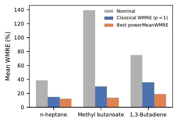
Tuning the power-mean objective’s own hyperparameters is itself the subject of a separate, companion methodology paper in preparation: a systematic search over the objective’s exponent and annealing schedule, combining a design-of-experiments response-surface search with a second, independent multi-optimizer confirmation pass, rather than hand-picking a setting once and reusing it. That manuscript is still in preparation, but its own figures — the toy objective-landscape comparison, the optimizer-comparison grid, the classical-WMRE dominance analysis, and the full ignition-delay and hyperparameter-sweep breakdowns across all three fuels — are shown further down this page, published ahead of the paper itself at the author’s own request (a deliberate, logged exception to the usual accepted-abstract-only tier; see DISCLOSURE_POLICY.md).

Extending to thermodynamic parameters

The correlation-aware, multi-stage philosophy developed here for kinetic rate parameters extends naturally to thermodynamic parameters (heat capacities, formation enthalpies) — the subject of a collaborative paper, led by Bishwajeet Singh with me as second author, under review at Fuel and separately accepted as an abstract for the 64th Symposium (Japanese) on Combustion, Fukuoka, Nov 2026 Singh et al. (2026). Per disclosure policy for work at this stage, only the title, authors and venue are given here — no formulae or numbers beyond what the accepted abstract itself already states publicly.

Results

(Published results only — see Disclosure Policy for why some numbers below are omitted.)

The multi-stage strategy applied to n-heptane is published: Panchal et al. (2023).

The power-mean objective work is accepted for presentation at the 64th Symposium (Japanese) on Combustion, Fukuoka, Nov 2026: Panchal and Narayanaswamy (2026). Per the accepted abstract, at an identical solver budget the power-mean objective reduces error to roughly a quarter of what classical WMRE achieves, across methyl butanoate and n-heptane case studies.

The underlying theoretical framework that makes this multi-stage, multi-dataset optimization computationally tractable is still in preparation; only the accepted abstract’s own claims are reproduced here.

From the hyperparameter-tuning paper draft

The figures below are from the in-preparation hyperparameter-tuning manuscript itself, shown ahead of publication (see the note above and DISCLOSURE_POLICY.md’s logged exception for 2026-09-08): the toy 2D landscape under classical WMRE vs. a fixed-p vs. an annealed-p power-mean objective, the same landscape searched by three different solvers, the classical-WMRE dominance analysis that motivates the whole approach, representative and full-appendix real ignition-delay fits across all three fuels, and solver-resolved hyperparameter-sweep heatmaps with real per-cell error numbers.

Validation

Solver cross-checks (genetic algorithm vs. gradient-based SLSQP, and vs. classical WMRE) confirm the multi-stage decomposition converges to physically consistent parameter sets rather than an artifact of the search method.

My contribution

Developed and led by me: the multi-stage decomposition and the power-mean objective function, under the supervision of Prof. Krithika Narayanaswamy. The shock-tube species-profile curve-capturing technique referenced alongside this work at the same symposium is separate, collaborative work led by Gautam Srikanth. The thermodynamic-parameter extension is separate, collaborative work led by Bishwajeet Singh, with me as second author.

Publications

• Panchal, Krunal; Vasudavan, Vaisakh; Narayanaswamy, Krithika (2023). A multi-stage kinetic reaction optimization strategy applied to n-heptane combustion mechanism. 14th Asia-Pacific Conference on Combustion (ASPACC).
• Panchal, Krunal R.; Narayanaswamy, Krithika (2026). A Power-Mean (Hölder) Objective Function for Balancing Unequal Datasets in Combustion Kinetic Mechanism Optimization: Case Studies on Methyl Butanoate and n-Heptane. 64th Symposium (Japanese) on Combustion. Accepted.
• Panchal, Krunal; Narayanaswamy, Krithika (2026). A multi-stage optimization strategy with partial polynomial response surfaces for combustion kinetic mechanisms. In preparation, target: Fuel.
• Singh, Bishwajeet; Panchal, Krunal; Narayanaswamy, Krithika; Ambikasaran, Sivaram (2026). A novel, temperature-dependent optimization framework for thermodynamic parameters of fuel kinetic mechanism. 64th Symposium (Japanese) on Combustion. Accepted.

Where this is going

A mechanism calibrated jointly across several fuels and datasets, without any one dataset silently winning the fit — and at a fraction of the solver budget a naive full-range optimization would need. More broadly, a systematic evaluation of fair multi-dataset objective-function design itself — comparing the power-mean approach against other candidate formulations under one shared framework — is an active research direction growing out of this work, still at the exploratory stage.