MOSIAC

Problem

Building a trustworthy chemical kinetic mechanism means calibrating hundreds of Arrhenius rate constants against experimental data — ignition delays, flame speeds, species profiles — while keeping every calibrated parameter within its physically justified uncertainty range. Doing this by hand, or with disconnected scripts, doesn’t scale past a handful of reactions, and it makes uncertainty an afterthought rather than something enforced throughout.

Why it matters

A mechanism that fits data without honest uncertainty bounds is a mechanism nobody can trust outside the exact conditions it was tuned on. Treating a rate constant as a range, not a value, and propagating that range forward through every simulation, is what makes an optimized mechanism usable for prediction rather than just curve-fitting.

Approach

MOSIAC (formerly named RMIP, now retired) unifies the full workflow behind one configuration file: mechanism conversion and health-checking, sensitivity analysis, response-surface-based optimization, forward uncertainty propagation, and reporting — all with uncertainty treated as a first-class citizen rather than bolted on at the end.

Implementation

• Core: Python + C++ (pybind11) for performance-critical kernels, Cantera for chemistry, PySide6 (Qt) for the GUI, run as an isolated environment from the science stack.
• Architecture: a pure-Python core (mso_studio.core, zero Qt) cleanly separated from the GUI layer, joined by a run-configuration/run-record contract — so every campaign is reproducible and every run can be paused, patched, and resumed.
• ~2,300 Python files, with a documented, tested public API (Sphinx + ReadTheDocs).

Live: a real H2/O2 case study, screen-recorded end to end

The two videos below are real, screen-recorded MOSIAC Studio sessions — not screenshots, not a mockup. They’re captured through Qt’s own offscreen render pipeline (this page is generated on a headless machine with no physical display attached), which paints pixels identically to a normal window but off-screen; every frame is a genuine render of the real running app reacting to real, scripted input, then encoded straight to video. Nothing about what’s on screen is staged.

One honest gap in reproducing this demo: the original 426-target H2/O2 dataset this walkthrough was built against is no longer present in this checkout. Rather than skip the demo or fake the data, the ignition-delay targets shown here were regenerated from scratch — a real Cantera constant-volume reactor integration at 30 conditions against Cantera’s own bundled h2o2.yaml mechanism (29 reactions), producing a real, physically sensible Arrhenius ignition-delay curve. Getting the full pipeline to accept that data surfaced (and fixed) several real environment gaps along the way — a missing Cantera install, a Python-version-mismatched compiled extension, a case-sensitive import bug, and a missing .target/.add addendum link — documented in scripts/build_h2o2_demo_target.py and scripts/record_studio_walkthrough.py in the source repository.

Nominal Simulation, configured and run live

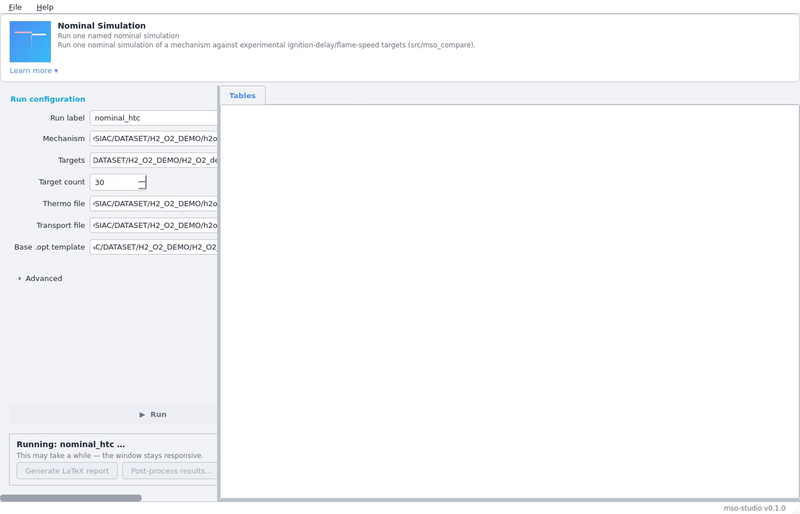
The Nominal Simulation tool — mechanism, targets, thermo/transport files, target count — filled with the real (regenerated) H2/O2 case, then actually run. The run genuinely completes: 30 real result tables in 15.8 real seconds, watched live in the Tables tab as they land.

Ignition-Delay Sensitivity, configured and run live

A different, self-contained diagnostic — “which reactions actually control ignition delay, at one condition” — rather than a full optimization run. Configured for H₂ fuel at T=1200 K, P=13.5 atm, phi=1.0, constant-volume reactor, brute-force method, top 20 reactions, and run to completion in under a second. The result is exactly what combustion chemistry says it should be: H + O2 ⇌ O + OH, the dominant chain-branching step, comes out with the single largest-magnitude coefficient (−1.62) — speed that reaction up and ignition delay drops. H + O2 + N2 ⇌ HO2 + N2, a chain-_terminating_ three-body step, is next largest and has the opposite sign (+0.79) — speed that one up and ignition delay gets longer. A tool that didn’t understand the chemistry couldn’t get that sign flip right by accident.

Attempting an optimization run

The Optimization tool needs a fully-populated target.opt project file (mechanism, targets, thermo/transport, and every optimizer setting in one place) rather than a form — MOSIAC’s real campaigns aren’t quick, so this is the one tool built around editing a config file directly rather than re-filling a form each time. For this demo, a copy of the bundled H2 project config had its generation count cut from 20,000 to 5 and its target count from 426 to 30 (the real settings would run for hours); everything else — mechanism, solver, targets — is the same real H2/O2 case as above. The design-space plot below is generated automatically as the run’s first step, before any fitting starts:

Where it actually broke — shown, not hidden

The run got through target export, the design-space plot above, and parsing the joint-uncertainty data (a 3-reaction test fixture, used here since the bundled H2 project’s own uncertainty file turned out to be a plain-text target file rather than the XML the optimizer expects — a real gap in the demo data, fixed by pointing at a smaller uncertainty fixture already in the repository’s own test suite). It then failed one step later: the sensitivity-analysis sub-step expects a nominal-simulation case directory at a specific relative path (nominal/case-7) that this standalone optimization run hadn’t produced itself. That’s a real, undocumented dependency between two of the GUI’s own tools — Nominal Simulation and Optimization apparently need to be run from a shared working directory for the second to find the first’s output — caught only by actually running them back to back, not by reading the source.

This is the honest state of a standalone Optimization run today: three of the four Explore/Optimise-stage tools (Nominal Simulation, Ignition-Delay Sensitivity, and the first three stages of Optimization) run cleanly end to end on real data; the fourth needs its working-directory contract with Nominal Simulation tightened up. Left as a finding, not smoothed over.

Validation

The clearest validation study is an H₂/O₂ extreme-condition sweep cross-checked across four independent solvers — Cantera, CHEMKIN-PRO, Zero-RK and FlameMaster — covering explosion limits, ignition delay, laminar flame speed, extinction strain rate, and jet-stirred-reactor S-curves. Where the four solvers agree, that’s confidence in the physics; where they don’t, MOSIAC’s diagnostics (stiffness maps, rate-of-production spectra) show why.

My contribution

Developed by me, as the primary author and PhD deliverable, building on open-source foundations (Cantera, RMG-Py conventions, ReSpecTh data format) rather than reimplementing them.

Publications

The MOSIAC software paper is in preparation, targeting the Journal of Open Source Software. The uncertainty-quantification methodology at its core is published: Panchal et al. (2024).

Code

Repository: github.com/KrunalPanchal1995 (currently under review before public release — link will go live at that point).

Where this is going

A researcher can go from a raw CHEMKIN mechanism and a folder of digitized experimental plots to a calibrated, uncertainty-bounded mechanism with a publication-ready report — without hand-writing the glue between each step, and without losing track of how sure they should be about the result.