MUQ-SAC — Joint Arrhenius Uncertainty Quantification

Problem

The three parameters of a modified-Arrhenius rate expression (pre-exponential factor A, temperature exponent n, activation energy Ea) are conventionally reported and perturbed as if independent — each given its own uncertainty factor, sampled on its own. They aren’t independent: a rate constant k(T) is one curve fit through experimental or theoretical data across a temperature range, and the three parameters trade off against each other along that fit. Treating them independently means a “3-sigma” A-factor combined with a “3-sigma” activation energy can correspond to a rate-constant curve dramatically outside anything the underlying data could ever support — an uncertainty region shaped like a box in parameter space when the physically valid region is a curved, correlated manifold. Sampling that manifold efficiently — without missing valid parameter combinations or wasting enormous compute exploring invalid ones — is the core difficulty MUQ-SAC addresses.

Approach

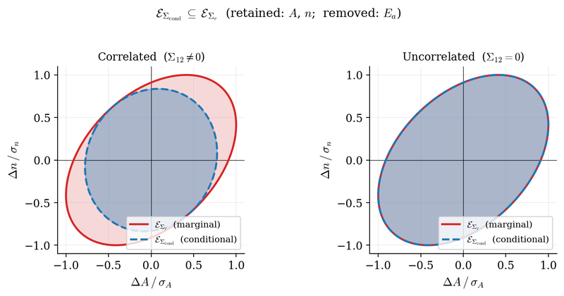
MUQ-SAC (Method of Uncertainty Quantification and Sampling of Arrhenius Curves) is a temperature-dependent, correlation-aware uncertainty quantification methodology: it characterizes the joint probability distribution of the Arrhenius parameters directly, as a region in (A, n, Ea) space, rather than three independent marginal distributions. Concretely:

• The valid joint-uncertainty region is represented as an ellipsoid in parameter space, derived from the correlation structure between the three parameters rather than assumed spherical.
• Every candidate sample is checked for containment within that ellipsoid before being accepted, and the ellipsoid can be projected down onto any 2D parameter subplane for visualization and for sampling strategies that operate in reduced dimensions.
• The method is benchmarked across four sampling-method classes for recovering the underlying curve fit — Class A (Moore–Penrose pseudo-inverse), Class B (SLSQP, full 3-parameter fit), Class C (ordinary least-squares, closed-form), and Class D (SLSQP, reduced 2-parameter fit / a matrix-based direct solve) — so the sampling result isn’t an artifact of one particular linear-algebra choice.
• Because the whole point is that parameters are correlated, the method is paired with a sensitivity-analysis-based correlation estimate: pairwise correlation heatmaps across A, n and Ea for a reaction set, used to decide which reactions’ parameters actually need joint (rather than independent) treatment.
• For the downstream optimization stages that consume this uncertainty, several response-surface surrogate forms (polynomial, Gaussian process, radial basis function) were compared for how faithfully each reproduces the true simulation response before picking one to build on.

Results

Published in Combustion Theory and Modelling (2024), applied to the H₂/CO kinetic mechanism: Panchal et al. (2024). The animated figure above shows all four sampling-method classes at once, real accepted Arrhenius curves building up their uncertainty bands in the same frame — with each panel’s own timer reading out the real measured compute cost of getting there, not a decorative counter. That cost turns out to matter a great deal: generating 100 samples measures at 204.3 s under Class B’s full 3-parameter SLSQP fit and 5.5 s under Class D’s reduced 2-parameter SLSQP fit, against 0.018 s (Class A) and 0.02 s (Class C) for the closed-form methods — roughly four to five orders of magnitude apart for statistically equivalent output on the same reaction family. That gap is the practical argument for the closed-form classes over the SLSQP-based ones at scale, not just a theoretical preference.

Validation

The sampling methodology is benchmarked across all four curve-generation classes (A/B/C/D above), with sampling-validity and projection checks confirming every sampled point respects the physically valid region — visualized directly in the ellipsoid-containment and projection figures above, not just asserted. Repeated independent sampling runs (the animated figure) are compared against each other as a convergence check: if a method were sensitive to random seed in a way that mattered, repeated runs would visibly disagree, and they don’t. The per-class timing was measured directly (time.perf_counter() around each sampler, not estimated), and reproduced independently for this page from the same saved sample data the original benchmark run produced.

My contribution

Developed by me as lead author, in collaboration with Vaisakh Vasudavan, Sivaram Ambikasaran, and my advisor Prof. Krithika Narayanaswamy — conceptualization, methodology, software and the primary formal analysis.

Publications

• Panchal, Krunal; Vasudavan, Vaisakh; Ambikasaran, Sivaram; Narayanaswamy, Krithika (2024). A fast uncertainty quantification methodology and sampling technique for joint probability distribution of the Arrhenius rate expression: a case study applied to H2/CO kinetic mechanism. Combustion Theory and Modelling 28, 411–440. doi:10.1080/13647830.2024.2326413

Where this is going

Rate-constant uncertainty that is sampled and reported honestly, correlation and all — the foundation MOSIAC’s optimization and forward-UQ stages build on.