All projects

  • sciml

Neural ODEs and Transformations — A Self-Built Course

A multi-month, derivation-first course on Neural ODEs, coordinate transformations and stiff chemical kinetics, with a verified animation for every session
98 images · 54 videos · 3 min read

Neural ODEs and Transformations — A Self-Built Course

datasheet // neural-ode-course

images
98
videos
54
formats
png, mp4
text
496 words · 3 min read
source
previous site
topics
  • p0 maps ×8
  • p1 transforms ×32
  • p2 ode theory ×16
  • p3 integrators ×22
  • p4 p6 neural odes ×33
  • p6 training and chemistry ×16
  • p7 objectives and gates ×10
  • p8 p9 capstones ×15

What this is

A personal, multi-month course I am building in the open to understand Neural ODEs properly: what a coordinate transformation does to a vector field, why stiff chemical kinetics breaks naive training, and how operator-theoretic ideas (Carleman, Koopman) and hard constraints fit on top. Every session is a full derivation (no skipped algebra), runnable Python, matplotlib figures, and a written document, and each one is organised by Bloom’s revised taxonomy from remembering up to creating.

Everything below is teaching material built on standard results. Each animation carries a numeric check that was actually run against it, listed in its caption.

Plan

Roughly 72 sessions from October 2026 to April 2027, foundations first. Fifty-two are written as of 6 October 2026; the next block is the constraint side (the stoichiometric matrix, conservation laws, hard constraints, CRNN).

Month Focus
Oct 2026 ODE theory, linearization, stiffness, first integrators
Nov Adaptive steps, change of variables, objective audit
Dec Neural-network recap, Neural ODEs, adjoint, regularization
Jan 2027 Stiff Neural ODEs, ChemNODE, objectives and power means
Feb Flows, slow manifolds, H2/air capstones, hard constraints, CRNN, reaction graphs, GNN+NODE
Mar Carleman, Koopman/DMD, PINNs, DeepONet, ACA, KAN, topology
Apr PyTorch, ONNX, quantization, synthesis

How the topics connect

  • Spine: ODE theory → integrators → change of variables → Neural ODEs → objectives → H2/air capstones.
  • Operator branch: the Jacobian from ODE theory leads to Carleman linearization, then Koopman, DMD and EDMD.
  • Constraint branch: stiffness leads to hard constraints and the stoichiometric matrix, then CRNN and SPIN-ODE, and separately reaction graphs and GNN+NODE.
  • Systems and operators: Neural ODEs also lead to PINNs, DeepONet, ACA, KAN and topology, and to PyTorch, ONNX and quantization.

Animations and figures

Grouped by phase: maps (P0), transformations (P1), ODE theory (P2), numerical integrators (P3), Neural-ODE core, adjoint and expressivity (P4 to P6, S028 to S037), and a last tab on regularization, stiff training, ChemNODE-style training on hydrogen/air, shooting and latent spaces, and flow maps (S038 to S042). Sessions S001 to S042. The videos loop silently; click a still figure for full size. Two further tabs cover the objective side (S043 to S046: power means, Sobolev loss, the Mahalanobis term, split estimators and leakage) and the capstones (S047 to S052: flows, slow manifolds, sparse and symbolic regression, the real hydrogen/air stiffness spectrum, state charts for a Neural ODE and a pilot check for training runs).

Method

  • Derive first. Each result is built from first principles before any code runs.
  • Verify every figure. Animations are produced by scripts that also write a verification.json of numeric checks, such as a measured convergence order against the theoretical one, or a conservation drift at machine precision.
  • Test the code. The course code base has an automated test suite that has to pass before a session counts as done.
  • State limits. Each session records claims written from memory that still need a source check.

The experimental setting behind the course, a stiff H2/O2 autoignition Neural ODE, is described in the Neural ODE playground project.

S001 What a Function Does to SpaceGrid morphing along a homotopy to a fold map; Jacobian sign tracked. Numeric check: max |det numeric - analytic| = 4.95e-10. Explain Calculus and transformations
S002 Smooth, Continuous, InvertibleFlow-map semigroup: phi_t then phi_s equals phi_(t+s). Numeric check: semigroup error 2.1e-14; order preserved. Explain Calculus and transformations
S003 Topological InvariantsTwo linked rings under an isotopy; Gauss linking integral tracked live. Numeric check: Lk stays in [-1.0009, -1.0003]. Explain Calculus and transformations
S004 Elementary Scalar TransformsPower map x^p as p sweeps; fixed and critical points. Numeric check: slope at x=1 error 1.4e-10; round trip 1.8e-15. Explain Calculus and transformations
S005 Exp, Log and the Log-ScalerMulti-scale trajectory as the log-scaler epsilon changes. Numeric check: round trip 1e-15. Explain Calculus and transformations
S006 Statistical TransformsEmpirical CDF, Box-Cox lambda and the Q-Q line. Numeric check: MLE lambda 0.011 vs scipy 0.0108. Explain Calculus and transformations
S007 Trig and Hyperbolic TransformsBounded maps saturate as the cloud scale grows. Numeric check: float64 tanh = 1.0 at x = 18.99. Explain Calculus and transformations
S008 Polar, Cylindrical, SphericalA path crossing the origin and the atan2 branch cut. Numeric check: jump = -2pi + 0.0318. Explain Calculus and transformations
S009 Curvilinear CoordinatesConformal homotopy from a Cartesian grid to elliptic coordinates. Numeric check: orthogonality deviation <= 3.7e-8 deg. Explain Calculus and transformations
S010 Linear Mapsexp(tA) of a non-normal matrix: transient growth. Numeric check: peak norm 2.563 at t = 0.663. Explain Calculus and transformations
S011 Homogeneous and Mobius MapsMobius flow through elliptic, parabolic, hyperbolic classes. Numeric check: cross-ratio drift 4.0e-15. Explain Calculus and transformations
S012 Polynomial BasesRunge function: equispaced vs Chebyshev nodes as degree grows. Numeric check: n=40 error 1.05e5 vs 2.89e-4. Explain Calculus and transformations
S013 Fourier and the DFTA sinusoid swept past Nyquist; the DFT peak jumps to the alias. Numeric check: peak bin = alias in 57 of 57 frames. Explain Calculus and transformations
S014 Laplace and ResolventsPoles moving with damping; time response and ROC. Numeric check: impulse response vs scipy 3.4e-13. Explain Calculus and transformations
S015 WaveletsHaar thresholding: kept coefficients vs error. Numeric check: error = discarded energy to 2.1e-14. Explain Calculus and transformations
S016 PCA and WhiteningCenter, rotate and whiten a correlated cloud. Numeric check: cond(cov) 14.62 -> 1.0. Explain Calculus and transformations
S017 Activation FunctionsReLU, tanh and softplus deforming a grid; Jacobian determinant mask. Numeric check: degenerate points after 2 layers: ReLU 87.3%, tanh 9.8%, softplus 0%. Explain Calculus and transformations
S018 Auditing a TransformationRaw vs transformed field; induced-field formula checked live. Numeric check: max error 1.3e-8 (log), 4.5e-9 (asinh). Explain Calculus and transformations
S019 ODEs and Vector FieldsParticle swarm in the oscillator field: exact vs Euler. Numeric check: Euler energy ratio 4.2844 = 1.0625^24. Explain Stiff systems and scientific ML
S020 Picard and GronwallPicard iterates converging to the exact solution. Numeric check: iterates equal Taylor sums. Explain Stiff systems and scientific ML
S021 Linearization and Phase PortraitsTrace-determinant point sweeping through the portrait zoo. Numeric check: Carleman N=1 equals Jacobian exactly (0.0). Explain Stiff systems and scientific ML
S022 Stiffness and ArrheniusROBER on the 3D simplex with its eigenvalue spectrum. Numeric check: sum drift 2e-15; hard-constraint drift <= 2.1e-14. Explain Stiff systems and scientific ML
S023 Forward Euler: Step HalvingEuler polygon converging to the exact curve as the step halves. Numeric check: global error slope 0.970 on log-log; local error slope 1.975. Explain Stiff systems and scientific ML
S023 Forward Euler: Stability Blow-upStep-size sweep on y' = lambda y: amplification factor 1 + h lambda crossing -1. Numeric check: measured amplification 0.5, -0.5, -1.5 equals 1 + h lambda. Explain Stiff systems and scientific ML
S024 RK4 Stages as Slope ArrowsThe four slope evaluations of one RK4 step and the weighted average that is taken. Numeric check: measured order slopes Euler 0.99, Heun 1.99, RK4 3.98; order-condition residual <= 3.9e-16. Explain Stiff systems and scientific ML
S025 Absolute Stability SweepThe point h lambda leaves the RK4 stability region while the live iterate blows up. Numeric check: RK4 real-axis bound 2.785293563 agrees across four methods to 1.3e-9. Explain Stiff systems and scientific ML
S026 Newton Inside a Backward Euler StepNewton iterations converging to the implicit-step solution on ROBER. Numeric check: step norms fall from 6.7e-4 to 2.2e-17 in 5 iterations. Explain Stiff systems and scientific ML
S026 BDF Steps on the ROBER SimplexVariable-order BDF steps filling the 3D conservation simplex. Numeric check: ROBER on [0,10] at rtol 1e-6: RK45 7088 steps, BDF 116. Explain Stiff systems and scientific ML
S027 Adaptive Step Size Chasing IgnitionStep markers and the step-size trace on a 3-reaction H2-like toy. Numeric check: own DOPRI5 vs SciPy RK45: identical accepted step counts in 6 of 6 runs. Explain Stiff systems and scientific ML
S020 Picard iteratesSuccessive Picard iterates for a polynomial ODE; each iterate adds a Taylor term. Explain Stiff systems and scientific ML
S021 The phase-portrait zooSinks, sources, saddles, spirals and centers from the trace and determinant of the Jacobian. Explain Stiff systems and scientific ML
S021 Carleman truncation ordersCarleman lifting at orders 1 to 4 compared with the true nonlinear solution; order 1 is the Jacobian linearization. Explain Stiff systems and scientific ML
S022 ROBER in 3DThe Robertson 3-reaction problem on its conservation simplex, coloured by log time. Explain Stiff systems and scientific ML
S022 Absolute stability regionsStability boundaries of explicit and implicit methods in the complex plane. Explain Stiff systems and scientific ML
S022 Hard vs soft conservationA soft penalty lets the species sum drift; the stoichiometric parametrization holds it to machine precision. Explain Stiff systems and scientific ML
S023 Euler on ROBER in 3DExact and forward-Euler orbits of the Robertson problem on its simplex. Explain Stiff systems and scientific ML
S024 Order-of-accuracy surfaceError against step size and method on a 3D surface. Explain Stiff systems and scientific ML
S025 Stability function surfaceThe modulus of R(z) over the complex plane with the contour at 1 that bounds the stability region. Explain Stiff systems and scientific ML
S026 BDF vs RK45 step pointsStep points of BDF and RK45 along the ROBER orbit in 3D. Explain Stiff systems and scientific ML
S027 Pseudospectrum surfaceResolvent norm surface of the ROBER Jacobian over the complex plane. Explain Stiff systems and scientific ML
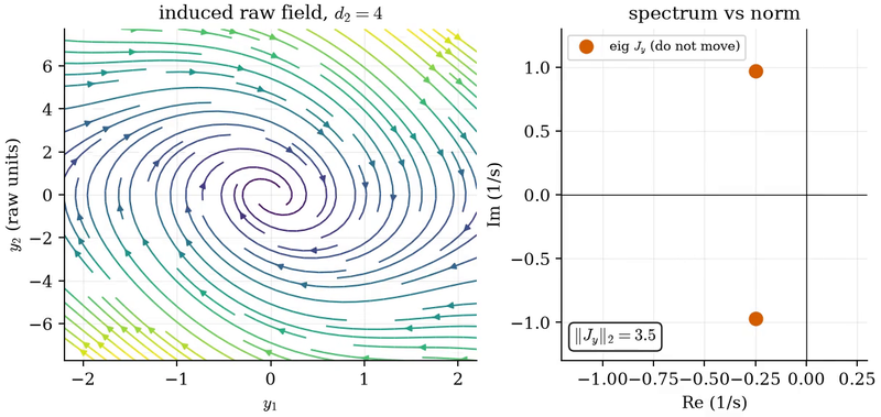
S028 Affine Normalization as Raw ReweightingInduced raw field as the second coordinate is stretched from d2 = 1 to 100, beside its Jacobian eigenvalues, which do not move. Explain Stiff systems and scientific ML
S029 SGD and Adam in Raw and Normalized CoordinatesFour descent runs on one quadratic loss: paths in the normalized plane and the four loss curves; the raw runs first move along one axis only. Explain Stiff systems and scientific ML
S030 Log-Scaler Dead Zone: clamp_min against add_epsPaths in the plane of log amplitude and log rate over the dead-fraction map; clamp_min paths stay where they start, add_eps paths reach the minimum. Explain Stiff systems and scientific ML
S031 The Price of Eigenvalue CompressionRaw and power-chart eigenvalues moving toward each other as the exponent p falls, with the error amplification 1/q for each mode. Explain Stiff systems and scientific ML
S032 Gradient Flow Across Depth as the Gain SweepsBackward signal norm layer by layer for one initialization gain at a time; blue where it vanishes, green balanced, red where it explodes. Explain Stiff systems and scientific ML
S033 Depth as Time: Residual Blocks Against the FlowSix initial conditions pushed through N tied residual blocks (N = 1 to 48) against the exact flow, with the mean end-point error falling like 1/N. Explain Stiff systems and scientific ML
S034 Neural ODE Training TrajectoriesTruth (solid) and learned field (dashed) in the phase plane and in time, logged at epochs 0 to 299 of a small training run. Explain Stiff systems and scientific ML
S035 Re-integrating the State BackwardsThe coupled system with s = 12, T = 2: the state re-integrated backwards leaves the true state and the error follows 1e-13 exp(s(T-t)). Explain Stiff systems and scientific ML
S036 Two routes to the gradient: the mismatch shrinks with the stepEuler path and the discretize-then-optimize and optimize-then-discretize gradients as the step is refined on Van der Pol. Numeric check: the discrete adjoint matches finite differences of the discrete loss to 4e-9; observed orders 1.06, 2.01, 3.98 for Euler, Heun, RK4. Stiff systems and scientific ML
S037 Augmented Neural ODE: Rings FlowLearned flow of the two-rings problem with one augmented dimension: the field carries the inner disk up and the ring down along u. Explain Stiff systems and scientific ML
S001 Jacobian parallelogram and determinant map Explain Calculus and transformations
S001 The fold map: two points to one Explain Calculus and transformations
S002 Flows cannot cross Explain Calculus and transformations
S003 Linked rings under a flow, linking number unchanged Explain Calculus and transformations
S003 Augmenting a dimension separates the annulus Explain Calculus and transformations
S004 Sign-power slope near the origin as the exponent changes Explain Calculus and transformations
S005 Clamp versus additive epsilon in the log-scaler Explain Calculus and transformations
S006 Box-Cox Jacobian slope near zero Explain Calculus and transformations
S007 Float64 round-trip error of bounded maps Explain Calculus and transformations
S008 Angle field and its branch cut Explain Calculus and transformations
S009 Four curvilinear coordinate grids Explain Calculus and transformations
S009 Toroidal coordinates in 3D Explain Calculus and transformations
S010 Shear flow: transient growth without an exponential rate Explain Calculus and transformations
S011 Mobius maps send circles and lines to circles and lines Explain Calculus and transformations
S011 Four Mobius classes and their iteration orbits Explain Calculus and transformations
S012 Runge phenomenon: equispaced against Chebyshev nodes Explain Calculus and transformations
S013 Aliasing: two sinusoids on the same samples Explain Calculus and transformations
S014 Resolvent gain of a non-normal matrix Explain Calculus and transformations
S015 Wavelet scale map of a two-bump signal Explain Calculus and transformations
S016 Centering, PCA rotation and whitening Explain Calculus and transformations
S017 Activation functions and their derivatives Explain Calculus and transformations
S018 Two transformed coordinates and their field derivatives Explain Calculus and transformations
S019 Phase portrait of the oscillator Explain Stiff systems and scientific ML
S020 Gronwall bound for a spiral, a saddle and Lorenz Explain Stiff systems and scientific ML
S021 Trace-determinant plane Explain Stiff systems and scientific ML
S021 Phase portraits of classic systems Explain Stiff systems and scientific ML
S022 ROBER trajectory over the stiffness surface Explain Stiff systems and scientific ML
S022 RK45 against BDF step counts on ROBER Explain Stiff systems and scientific ML
S023 Euler polygons approach the exact curve as h halves Explain Stiff systems and scientific ML
S023 Forward Euler energy growth on the oscillator Explain Stiff systems and scientific ML
S024 Measured order of accuracy of one-step methods Explain Stiff systems and scientific ML
S024 Work-precision of explicit Runge-Kutta methods Explain Stiff systems and scientific ML
S025 Stability regions of explicit methods Explain Stiff systems and scientific ML
S025 Stability ceiling of the step size along ROBER Explain Stiff systems and scientific ML
S026 BDF stability regions Explain Stiff systems and scientific ML
S026 L-stability: trapezoid ringing against backward Euler Explain Stiff systems and scientific ML
S027 Step-size controller on Van der Pol Explain Stiff systems and scientific ML
S027 Cost against tolerance for adaptive solvers Explain Stiff systems and scientific ML
S028 Induced raw field as one coordinate is stretched Explain Stiff systems and scientific ML
S028 RK4 commutes with affine maps, not with log Explain Stiff systems and scientific ML
S028 Conditioning of raw and normalized MSE Explain Stiff systems and scientific ML
S029 SGD and Adam, raw and normalized: four ways to descend Explain Stiff systems and scientific ML
S029 Iterations against scale ratio for SGD and Adam Explain Stiff systems and scientific ML
S030 ROBER in log coordinates Explain Stiff systems and scientific ML
S030 Dead zone of the clamp: loss contours and convergence maps Explain Stiff systems and scientific ML
S031 Power chart: eigenvalue compression and its price Explain Stiff systems and scientific ML
S031 Smooth charts and the spectral radius along a trajectory Explain Stiff systems and scientific ML
S032 Gradient flow against depth and gain Explain Stiff systems and scientific ML
S032 Optimizers as integrators Explain Stiff systems and scientific ML
S032 Optimizer race on a small tanh network Explain Stiff systems and scientific ML
S033 Effective weight decay and reparametrization Explain Stiff systems and scientific ML
S033 Depth as time: residual blocks against the flow Explain Stiff systems and scientific ML
S034 Anatomy of a Neural ODE forward pass Explain Stiff systems and scientific ML
S034 Spectral radius and largest relative rate on ROBER Explain Stiff systems and scientific ML
S035 Adjoint sensitivity on Van der Pol Explain Stiff systems and scientific ML
S035 Instability of re-integrating the state backwards Explain Stiff systems and scientific ML
S036 Two routes to the gradient Explain Stiff systems and scientific ML
S036 Discretize-then-optimize against optimize-then-discretize Explain Stiff systems and scientific ML
S037 The reversal map that a flow cannot represent Explain Stiff systems and scientific ML
S037 Exact lift of the rings problem Explain Stiff systems and scientific ML
S037 Learned decision regions with augmentation Explain Stiff systems and scientific ML
S038 Regularizing Neural ODE dynamics: paths straighten as the Jacobian weight grows70 test points of the planar twist map flowing through six learned fields as the Jacobian weight grows from 0 to 1. Numeric check: inference NFE 38 to 20; kinetic energy at or above its chord bound at all 512 test points of four models. Stiff systems and scientific ML
S039 Stiff Neural ODE on ROBER: training with backward Euler in the loopBackward-Euler path of a ROBER Neural ODE against the Radau reference during training, epochs 0 to 299. Numeric check: re-integrating the learned field with Radau gives 0.96 to 1.11 times the training loss in 22 of 27 runs. Stiff systems and scientific ML
S040 ChemNODE-style training on H2/air autoignition: a held-out conditionA ChemNODE-style Neural ODE (log chart) on the held-out condition T0 = 1125 K against Cantera. Numeric check: elemental mass drift of the exact reference below 1e-8; reference ignition delay 7.3e-5 s. Stiff systems and scientific ML
S041 Single shooting flattens out; multiple shooting follows the oscillationSingle shooting (left) and windows of 10 intervals (right) on six periods of an oscillator, epochs 0 to 999. Numeric check: full-horizon MSE 0.46 to 0.48 for single shooting against 1e-4 to 1e-3 for windows over three seeds. Stiff systems and scientific ML
S042 A learned flow map rolled out on a held-out ignitionA learned flow map (scaled chart, POD latent space of 5) rolled out in 150 steps on the held-out condition 1125 K. Numeric check: elemental drift 1.4e-14; semigroup defect of the exact map 3e-16. Stiff systems and scientific ML
S038 The twist map learned four ways: paths and deformed gridsTest trajectories and the learned map applied to a grid for no penalty, a kinetic penalty and two Jacobian penalties. Numeric check: inference NFE 38, 26, 26, 20; median path straightness 0.915 to 0.992. Stiff systems and scientific ML
S038 Loss against inference cost for kinetic and Jacobian penalties42 runs on the planar twist map: validation loss against inference NFE, and what each penalty buys and costs. Numeric check: Spearman rank correlation of NFE with J 0.92 and with K 0.79. Stiff systems and scientific ML
S039 Amplification factors: backward Euler contracts an unstable modePer-step multiplier of the exact flow, backward Euler, forward Euler and RK4 against h*lambda. Numeric check: z = 5 gives -0.25 for backward Euler against e^5 for the exact flow. Stiff systems and scientific ML
S039 Failure map of an explicit solver on random initial fieldsFraction of 12 random fields per cell on which RK45 finishes, ends in blow-up or at the step cap, and on which backward Euler stays bounded. Numeric check: all 22 failing cells contain blow-ups; the step cap is reached in 2. Stiff systems and scientific ML
S039 Gradient clipping against no clipping on ROBERFinal loss, loss curves, gradient norm and learned spectral radius with and without clipping the gradient norm at 1. Numeric check: final loss 2e-4 to 1e-3 against 7e-3 to 2.8e-2 (8 of 9 runs finish). Stiff systems and scientific ML
S040 Stiffness and the explosive mode of the real H2/air JacobianEigenvalues of the true Jacobian along a Cantera autoignition from 1000 K. Numeric check: spectral radius up to 8.3e8 1/s; explosive mode up to 2.96e5 1/s at t/tau = 0.991. Stiff systems and scientific ML
S040 A held-out and an extrapolation condition: temperature, OH and element balanceLearned models against Cantera at 1125 K (held out) and 950 K (extrapolation). Numeric check: elemental drift of the trajectory-trained models 13% to 159%; the derivative-matched model leaves the plot. Stiff systems and scientific ML
S041 Loss landscape of single and multiple shooting (closed form)Exact rotation model: loss against the model rate for several horizons and window lengths, and the basin of attraction against length. Numeric check: basin half-width 0.743 rad/s measured against 4.493/T = 0.749 at T = 6 s. Stiff systems and scientific ML
S041 POD of the chemistry snapshots in three chartsSingular values, captured energy, reconstruction error and elemental change after decoding for the scaled, Box-Cox and log charts. Numeric check: rank 7 in the scaled chart; elemental change 6e-14 for every rank. Stiff systems and scientific ML
S042 Step-size robustness of learned flow mapsDelay error against the number of rollout steps, spread of the final temperature, and the semigroup defect for pair-only maps and maps with the n-step rollout loss. Numeric check: detector resolution 3/N of the delay. Stiff systems and scientific ML
S042 Learned flow maps rolled out on held-out conditions600-step rollouts at 1125 K and 950 K for the best seed of four models, with the hydrogen element balance. Numeric check: scaled latent map elemental drift 1.4e-14. Stiff systems and scientific ML
S043 Hölder means: which channel the gradient pushes on as the exponent changesClosed-form replay of nine channel errors through a family of power means, from p = 40 to p = 0.03: at large p the whole weight sits on the largest error, at small p on the smallest. Numeric check: the level set of the mean through the point and the weights of its steepest-descent step are computed from the same formula in every frame. Stiff systems and scientific ML
S044 A model of OH with a Sobolev term: value, time derivative and gradient share through trainingOH from a hydrogen/air ignition fitted with a value term and a derivative (Sobolev) term, weight 100, at six epochs. Numeric check: the norm share of the fit term falls from 0.86 to about 0.01 and ends at 0.48. Stiff systems and scientific ML
S045 The Mahalanobis ellipse of two correlated errors as the shrinkage is removedStandardized errors of H and O (measured correlation 0.95) with the unit ellipse of the Mahalanobis distance for shrinkage from 1 to 0.001. Numeric check: the squared distance of a unit error against the correlation grows from 1.00 to 17.92 while along it falls to 0.51. Stiff systems and scientific ML
S046 Re-drawing a split until it looks good: what a gate would reportError of 24 condition-blocked splits inside the training hull and the running minimum a gate would report as more splits are tried. Numeric check: honest risk 0.0171 (mean of all 24 splits); the best of 24 reports 0.0049. Stiff systems and scientific ML
S047 A continuous normalizing flow carries a Gaussian to the two-moons dataDensity on a grid and carried base samples (colour: log density of each particle) from t = 1 to t = 0 for a trained continuous flow. Numeric check: test negative log-likelihood 1.82 nats for the exact-trace flow and 1.84 with Hutchinson, seed 0. Stiff systems and scientific ML
S048 160 starting points fall onto the slow manifold of the Davis-Skodje modelSlow manifold of a two-variable fast-slow system with the quasi-steady-state and ILDM approximations, and the median distance to the exact manifold. Numeric check: the distance decays as exp(-gamma t) with gamma = 10 down to 1e-7. Stiff systems and scientific ML
S049 Sparse regression: the threshold sweeps from 12 terms to the exact 8-term supportSTLSQ on a three-species kinetics problem: normalized contribution of each library coefficient against the threshold. Numeric check: the exact 8-term support is recovered at threshold 2.7e-4; spurious terms are red. Stiff systems and scientific ML
S050 The nine Jacobian eigenvalues of a hydrogen/air ignition against the RK4 stability regionEigenvalues in the complex plane (symmetric-log axes, explosive eigenvalue in red) and the same multiplied by a fixed step against the RK4 region, T0 = 1000 K, 1 atm. Numeric check: h times the spectral radius is 97 at t = 0 and 1.6e4 at 1.6 tau, against the stability limit 2.785. Stiff systems and scientific ML
S051 The decoded temperature of a held-out ignition during training in four state chartsNeural ODE trained in the raw, scaled, log and POD charts (seed 0, backward Euler in the loop), decoded to temperature at epochs 0 to 599 against Cantera at 1125 K. Numeric check: final interpolation nRMSE 0.27 (POD), 0.40 (scaled), 0.47 (log), 202 (raw), medians of three seeds. Stiff systems and scientific ML
S052 72 training runs through a pilot check: who passes at each epoch, and who ends wellEach point is a run in the plane of a run-health score and the H2O peak-height error; inside the dashed box a run passes the pilot check. Green: healthy at the end, red: not. Numeric check: no run passes at epoch 0; 34 of 72 end healthy. Stiff systems and scientific ML
S044 The fit and Sobolev gradients of one parameter cross as training proceedsGradient of the value term and of the derivative term for y' = a y against the model rate, their ratio, and the fit share along two training runs. Numeric check: the two gradients are equal near a = -0.65 and both vanish at the true rate a = -1. Stiff systems and scientific ML
S044 Measured gradient shares of the fit and Sobolev terms for a hydrogen/air modelGradient norms and the norm and projection shares of the fit term for weights 1 and 100 (seed 0). Numeric check: the norm share ends at 0.48 for both weights; the projection share ends at 0.16 and 0.07. Stiff systems and scientific ML
S045 Mahalanobis geometry of two correlated species errorsUnit ellipses for HO2-H2O2 (correlation 0.61) and H-O (0.95) and the weight ratio (1+rho)/(1-rho). Numeric check: 4.1 and 35.5. Stiff systems and scientific ML
S045 The correlation matrix of the species errors has two zero eigenvalues: the element lawsEigenvalues of the correlation matrix, the weights 1/lambda with shrinkage, and the variance along the two conservation laws. Numeric check: the two smallest eigenvalues are 1e-16 and 1e-18 of the largest; the laws have variance 1e-18 and 1e-17 of the total. Stiff systems and scientific ML
S046 Error of a split against the choice of held-out conditionsCondition-blocked splits of 11 conditions holding out 4, 6 or 8: all held-out conditions against those inside the hull, and the spread between splits and between seeds. Numeric check: three seeds per split, 24 splits per size. Stiff systems and scientific ML
S046 Measured leaks: random against blocked splits, and normalizers that see the test setGeometric-mean nRMSE for random-sample and condition-blocked splits, the error by time window and two leaky normalizers, one line per seed. Numeric check: random-split R-hat 0.021 against 0.011 on three new conditions. Stiff systems and scientific ML
S047 Learned densities of Real NVP and continuous flows on three data setsTwo moons, two rings and a checkerboard with the density of a coupling flow, an exact-trace flow and a Hutchinson-trace flow (seed 0). Numeric check: test NLL 1.804, 1.819, 1.844 (moons); 2.643, 2.641, 2.680 (rings); 2.475, 2.360, 2.389 (checkerboard). Stiff systems and scientific ML
S047 Negative log-likelihood, cost and learning curves of the three flowsTest NLL for three seeds, total function evaluations, and validation NLL against cumulative NFE on two moons. Numeric check: the coupling flow uses about 7e3 evaluations, the continuous flows about 4e4. Stiff systems and scientific ML
S048 The real Jacobian spectrum of hydrogen/air through ignition and the number of exhausted fast modesNine eigenvalues at 1000 K and 1200 K and the exhausted-mode count at three tolerances. Numeric check: explosive mode 4.45e4 1/s at half the ignition delay, peak 3.09e5 at 0.988 tau; the count goes from 2 to 5. Stiff systems and scientific ML
S049 Symbolic regression on an Arrhenius law: Pareto fronts, a correlated pair and the extrapolationPySR Pareto fronts at 1% noise, the correlation of the fitted exponent and activation energy over 2000 noise draws and the maximum relative error of four forms outside the fit range. Numeric check: correlation -0.999; extrapolation errors 0.0055, 0.14, 0.63 and 1.8. Stiff systems and scientific ML
S049 Sparse regression in a POD latent space of the ignition: a good derivative fit, a failed rolloutSingular values of the scaled ignition, the relative derivative error of degree-2 and degree-3 models, and their rollouts. Numeric check: derivative error 3e-8 at 6 modes and degree 3; all four rollouts stop before ignition, at 0.13 to 0.93 tau. Stiff systems and scientific ML
S050 The spectral radius of hydrogen/air along 24 ignitionsLargest decay rate of the Jacobian against t/tau for four initial temperatures, three equivalence ratios and two pressures. Numeric check: peak 1.08e8 to 1.58e10 1/s, a factor 147; the front multiplies it by 2 to 178. Stiff systems and scientific ML
S051 The spectral radius of the true field in five state chartsInduced spectral radius at 1000 K and 1300 K and the ratio to the raw chart at t = 0. Numeric check: raw and scaled agree to 1e-8; the log chart is inflated only at t = 0 (x1.7 at 1125 K to x33 at 1300 K). Stiff systems and scientific ML
S051 Physical-state error of a Neural ODE in five charts and two lossesFinal nRMSE, three seeds, interpolation and extrapolation conditions, trajectory loss against derivative matching. Numeric check: POD 0.27, scaled 0.40, Box-Cox 0.45, log 0.47, raw 202 (trajectory loss, medians). Stiff systems and scientific ML
S052 No chart compresses the stiffness ratio of hydrogen/air; a nonlinear chart moves a spectrum only away from restStiffness ratio in five charts against the power-compression targets, the effective exponent against T0, and a toy system. Numeric check: effective exponent 1.00 for raw, scaled and POD, 0.86 for log; toy spectrum ratio 0.92 to 1.09 at distance 1. Stiff systems and scientific ML

How to recreate this plot

Watch

A short screen capture of the Math Visualization Studio. Each step is captioned in the clip.

Steps

  1. Open the controls panel
  2. Choose the example: a map u(x, y), v(x, y)
  3. Choose the shape: circle
  4. Raise the window half-width to 4
  5. Press Play

Code and PDF notes

Free of cost. I approve each request and reply by email.

To request the files, email me at and mention the item id. project-neural-ode-course