Scientific ML for Stiff Kinetics

Problem

H₂/O₂ autoignition is a deceptively small test case for a neural surrogate: eight species, nineteen reactions — and a stiffness ratio spanning five to eight orders of magnitude, radical species that behave as transient quasi-steady-state spikes rather than smooth trajectories, and eight decades of dynamic range across species concentrations. A “tiny” mechanism turns out to be one of the harder regimes to learn.

Approach

This is an ongoing, unpublished research effort — two NeurIPS 2027 submissions are in preparation from it, so the specific architecture and its exact results are withheld here pending submission. What I can share is the shape of the investigation: a long, honestly-documented sequence of architectural generations, moving from naive direct-time neural ODEs, through reparameterized time coordinates and physics-constrained formulations, to representation-level fixes for the underlying stiffness — each generation motivated by a specific, diagnosed failure of the one before it, with negative results kept in the record rather than discarded. The gallery includes both the current best result (labeled “champion” — architecture and exact numbers withheld) and an earlier intermediate checkpoint (labeled “journey”), shown alongside each other deliberately rather than only publishing the winner.

Diagnosing training pathologies, not just watching the loss curve

A loss curve alone doesn’t say why a model is struggling. One recurring diagnostic across this search: instrument the network’s first layer directly and check whether it’s saturating — a classic vanishing-gradient failure where a tanh activation gets pushed so far into its flat regions that gradients barely flow back through it. Run across sixteen single-variable versions of the same architecture (each version changing exactly one thing from the last), the pattern is stark: every version training directly in raw physical units saturates fully, while the versions built on a per-channel [0,1] normalization never do. Not every architecture change in this search mattered — this one did, and instrumenting the layer directly is what showed it, rather than inferring it indirectly from a loss curve that looks similar either way.

The discipline that mattered most

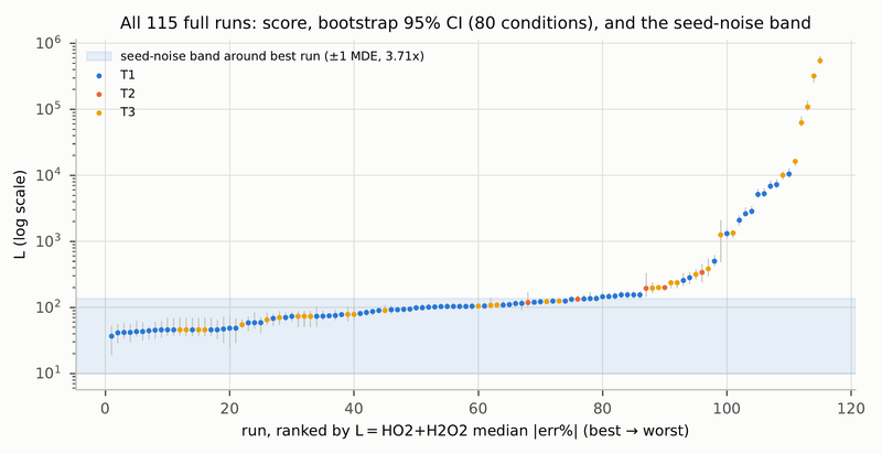
The most consequential step wasn’t a bigger model or more training — it was stopping to statistically audit my own results before believing them. A controlled, multi-seed re-analysis of the full 115-run experimental campaign found that 67% of runs (77 of 115) fell inside the seed-noise band of the single best result — the same configuration, re-run with a different random seed alone, produced up to a 3.4x spread in the reported metric. At the sample sizes this campaign actually used, the minimum effect size detectable at conventional statistical power was a 3.71x (271%) fold-change — anything smaller than that could not have been distinguished from noise regardless of whether it was real. A separate check found the training objective actually being optimized correlated only weakly with the metric the results were ultimately judged on (Spearman ρ ≈ 0.13) — a substantial share of the campaign’s compute was spent optimizing a proxy that wasn’t a reliable stand-in for the thing that mattered. That distinction — which apparent wins are real and which are noise — is now a standing check applied before any result from this line of work is reported as fact, here or in the eventual papers.

Recurring lessons (method-agnostic, safe to share)

• Reparameterize the independent variable before touching the network architecture.
• Make physics constraints structural — build them into the representation — rather than penalizing their violation after the fact.
• Budget explicitly for gradient amplification when training through multi-step rollouts.
• A win on one metric does not automatically compose with a win on another; each combination has to be re-verified, not assumed.
• Statistical rigor about your own results is not optional once a claim will be published.
• A reproducibility gate pays for itself: a later re-porting pass across this campaign’s architecture families required every migrated version to reproduce its original’s own training-loss history bit-for-bit at default settings before any new capability was considered done — catching silent behavior drift at the moment it’s introduced, not months later when it’s hard to trace back.

A published-paper replication, done honestly

Separate from the unpublished architecture search above, and safe to detail in full since it reproduces someone else’s already-published method rather than my own unpublished one: a from-scratch replication of Kumar, Kumar & Pal (2025), “A physics-constrained neural ordinary differential equations approach for robust learning of stiff chemical kinetics,” Combustion Theory and Modelling 29(3), also on arXiv as 2312.00038. The paper trains a NeuralODE surrogate (NODE) for stiff H₂/air autoignition and shows that adding an elemental mass-conservation penalty to the loss (PC-NODE) produces a model that’s both more physically consistent and, empirically, easier to train. This replication reproduces the paper’s network architecture, loss formulation and training/validation grid exactly (see the project’s own component-by-component comparison against the paper), substituting three things the paper’s own repository doesn’t distribute — training used Adam rather than the paper’s full-batch Levenberg-Marquardt, a fixed-step solver rather than the paper’s stiff implicit integrator, and Cantera’s bundled H₂/O₂ mechanism rather than the paper’s specific uncited one — each substitution stated up front rather than silently made.

At the checkpoints saved so far (33 epochs for the baseline NODE, 3 for PC-NODE — early, not final), neither model has converged onto the ignition trajectory yet, and the result on the paper’s own headline comparison is genuinely partial: PC-NODE drifts less than the unconstrained baseline for the H element, matching the paper’s claim, but not yet for O. That’s reported as-is rather than rounded off to “it worked” — the same discipline applied to the unpublished work above.

Validation

Every architecture generation was checked against a Cantera ground truth across a held-out condition set, and the final statistical audit re-examined the entire multi-run campaign for seed sensitivity before any headline number was treated as trustworthy. The PC-NODE replication is checked the same way: against its own Cantera-generated ground truth, with the paper’s own reported metrics as the standard it’s compared against, not an internally chosen one.

My contribution

Sole researcher on this line of work; developed from scratch, including the custom transforms, physics-constraint formulations, and the statistical audit methodology itself. The PC-NODE replication is my own independent reproduction of Kumar, Kumar & Pal’s published method — not a co-authored or adapted codebase.

Where this is going

Two forthcoming NeurIPS 2027 submissions, and — more durably — a working discipline for telling a real improvement apart from noise before publishing it.