Turbulence Closures — From Mixing Length to Data-Driven RANS

Problem

Turbulence closure is the central open problem in practical CFD: DNS resolves turbulence exactly but is computationally infeasible at engineering scale, so every practical solver leans on a modeled closure — and a closure’s accuracy, applicability range, and failure modes have to be understood on purpose, not assumed because a commercial tool ships it as a menu option. Most CFD users pick a turbulence model as a black-box setting; this project instead builds the field’s entire lineage from scratch, in a testable Python sandbox with an honesty discipline enforced by code, not just convention — feeding directly into PANSOPHIA’s own from-scratch turbulence module.

Approach

A chronological curriculum, one pluggable closure contract (ClosureModel, a single method mu_t_field, generalized to also host Reynolds-stress-transport models with no scalar eddy viscosity at all): Prandtl’s (1925) mixing length through one-equation (Spalart-Allmaras) and two-equation (k-ε, k-ω/SST) RANS models, Reynolds-stress transport (SSG, 1991), a nonlinear eddy-viscosity model (Shih-Zhu-Lumley, 1993), v2f (Durbin, 1991/1995) — 17 closures built and registered, covering the field from 1925 to 1997 in full. Then genuinely past classical RANS: a real unsteady 2D incompressible Navier-Stokes solver (vorticity-streamfunction, pseudo-spectral, validated against the closed-form Taylor-Green vortex and an inviscid energy/enstrophy conservation check) hosting LES sub-grid closures (Smagorinsky, dynamic Smagorinsky, WALE), a hybrid RANS-LES method (DES97, Spalart et al. 1997, built as a direct modification of Spalart-Allmaras’s own wall-distance length scale), and a first data-driven closure correction — a closed-form curve fit (not a trained model) against DNS data, with a genuine train/test split.

Every closure is checked against a BenchmarkEntry registry that mechanically requires a disclosed caveat for anything short of a clean pass (the constructor itself refuses to build an entry with a "finding" or "miss" outcome and no caveat) — a validation dossier with no misses in it is not a validation dossier.

Results

LES on a genuine 2D solver (Fig. 1–3): a Smagorinsky sub-grid closure cuts the coarse-grid spectral energy-pileup error by 3.3x against a DNS reference tuned to hit the theoretical $E(k)\sim k^{-3}$ enstrophy-cascade slope almost exactly (measured slope −3.033); the accompanying video shows the classic 2D-turbulence signature of same-signed vortices merging over time while enstrophy cascades to small scales and dissipates.

Hybrid RANS-LES (Fig. 4): DES97 matches plain Spalart-Allmaras’s own wall shear stress to ~9 significant figures exactly where its RANS branch is supposed to stay active — and, just as importantly, the outer-region limitation of running a 1D closure with no real LES grid behind it is measured and disclosed (a ~92x eddy-viscosity collapse), not hidden.

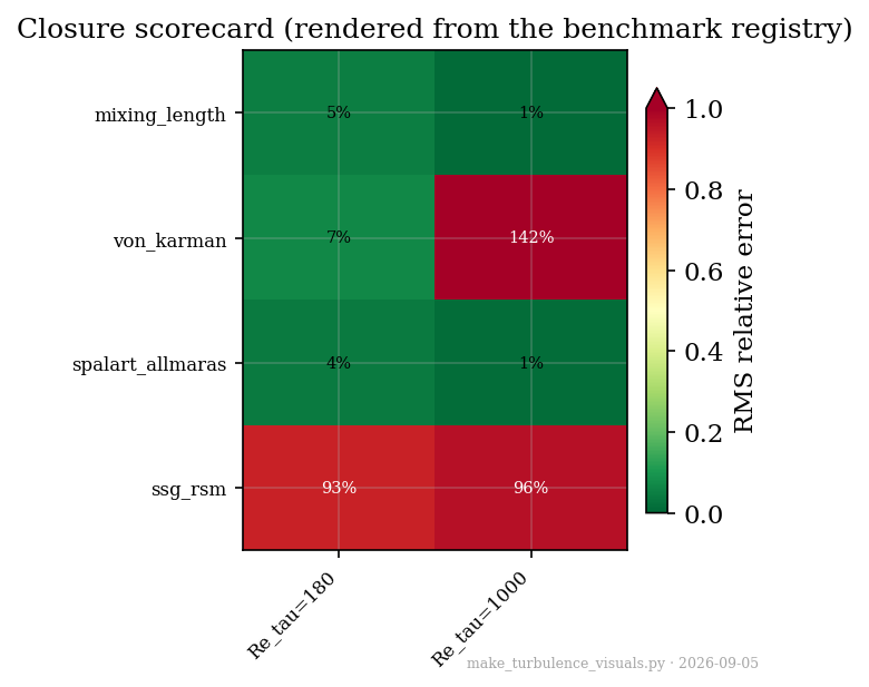
Reynolds-stress transport vs. DNS (Fig. 5): SSG’s mean-velocity profile misses Lee-Moser channel DNS by 93–96% RMS — a genuine, large, disclosed miss, reported at the same standard as every passing result, because a closure that only shows its wins isn’t validated at all.

A first data-driven closure (Fig. 6): a $C_\mu(y^+)$ correction curve-fit against $\mathrm{Re}_\tau$=180 DNS, evaluated — never re-fit — against held-out $\mathrm{Re}_\tau$=1000: a genuine 52% RMS generalization miss, with the root cause ($\mathrm{Re}_\tau$=180’s own short log-law window biasing the fitted asymptote) investigated and recorded, not just measured and dropped.

Turbulent-kinetic-energy budget, order-of-magnitude analysis (Fig. 7): the production/ dissipation/transport balance directly from Lee-Moser DNS, the physical structure every RANS closure in this study approximates — production peaks sharply in the buffer layer, dissipation dominates all the way to the wall, and pressure-strain integrates to exactly zero for the scalar TKE budget by construction (it only redistributes energy between Reynolds-stress components, which is exactly why the Reynolds-stress-transport model in Fig. 5 has to model it explicitly).

A general-purpose turbulence visualization/video toolkit, built afterward and exercised against this same study’s own data: Okubo-Weiss coherent-structure segmentation, Q-criterion, line integral convolution, a real (not model-spectrum) energy spectrum and spectral energy flux showing 2D turbulence’s dual inverse-energy/forward-enstrophy cascade directly, structure functions, velocity-gradient-invariant statistics, and a closure scorecard rendered straight from the benchmark registry, quadrant analysis, and a two-point spatial autocorrelation with its own integral length scale. Six invented visualization techniques get their own video/figure treatment — an “Instrument Panel” dashboard synchronizing a field, its live spectrum, and an energy/enstrophy time history under one moving cursor; a “Scale Telescope” that sweeps a band-pass window through wavenumber space instead of through time; a “Closure Divergence Theatre” watching two SGS models diverge from an identical initial condition; a “Backscatter Flash Map” reconstructing the spatial structure behind up-scale energy transfer at every frame; an “Anisotropy Painting” mapping Reynolds-stress state to a color ribbon; and a “Budget Residual Field” showing a closure’s own local self-consistency node by node. A verification pass — actually looking at every rendered frame, not just checking for a clean exit code, across two build passes — caught and fixed eight real bugs this way, including a sign error in the spectral-flux computation that an energy-conservation check alone structurally could not detect. One figure reports a genuine negative result, kept in rather than swapped for a cleaner case: the Budget Residual Field technique has a real, disclosed limitation applying it to a relaxed-Picard RANS solve (full account in the project’s own lab notebook).

A ParaView-class data pipeline and a telemetry subsystem (Fig. 12–15 + video), built after a direct measurement found the study persisted zero numbers anywhere — every result existed only as a formatted string, recomputed from scratch on every import. RunLogger now instruments the solvers (additive, opt-in, verified bit-identical to the pre-instrumentation code when unused — 18 checked configurations, 0 mismatches) and logs both individual per-node values and collective statistics (min/max/rms/percentiles, an exponent histogram, dynamic-range-in-decades) to Parquet/HDF5, ML-training-ready with a self-describing schema. A new FieldDataset/TimeSeries data model plus calculator/gradient/divergence/curl/slice/clip/threshold/contour/ glyph/stream_tracer/temporal-statistics filters, and VTK-XML writers (.vti/.vtr/.vtu/ .pvd, plus XDMF+HDF5 for long series) give this study’s data a genuine source-to-filter-to-view pipeline for the first time; Animation turns a TimeSeries into a movie in three lines instead of a bespoke FuncAnimation script per video. Three more invented visualization techniques ride directly on the new telemetry: a Magnitude Cascade Ledger (every term of a real Picard iteration’s own balance on one shared log-magnitude axis, dominance switches highlighted), a Vanishing Horizon (a residual’s own decay against two genuinely distinct thresholds — float64 denormal extinction versus mere irrelevance relative to the equation’s own dominant scale), and a Decade-Band Field Map (a field rendered in discrete power-of-ten bands) — the last of which produced a real caught-before-trust finding: a first-draft caption assumed “vortex cores several decades above background,” which did not survive actually looking at the rendered image (the dominant visible structure is the field’s own vorticity zero-crossing topology instead), fixed to describe what the figure actually shows.

Validation

17/17 cataloged closures built and registered; 56 BenchmarkEntrys (covering the closures above plus previously-uncovered infrastructure — grid/linear-algebra primitives, near-wall treatment, boundary-layer integral quantities — closed in an earlier session), every one now carrying a machine-readable results_json record (closing a real, measured gap: this field existed since the study’s first session but was populated on 0 of 56 entries until this one), zero silently-hidden misses — the registry’s own constructor forbids that. Every model is checked against a closed-form solution, DNS (Lee & Moser channel data), or a cross-check reference — never against a hand-picked “looks right” snapshot. The visualization toolkit’s own derived- quantity functions carry their own closed-form/conservation-law test suite (20 tests, including a new directional-anisotropy check that closes a previously-disclosed gap), independent of the closure registry above; the new pipeline/telemetry infrastructure carries 40 more tests of its own (writer round-trips, XML well-formedness, a sphere isosurface area converging to $4\pi r^2$, and the rendered-figure-level checks behind the three new techniques above).

My contribution

Designed and built the entire closure contract, solver stack, and the mechanically-enforced disclosure registry from scratch; ported the classical closures and independently re-derived the LES/hybrid/data-driven methods (Smagorinsky and WALE cross-checked character-for-character against PANSOPHIA’s own production Julia implementation; dynamic Smagorinsky re-derived from the Germano-Lilly identity). Development used Claude.ai as a coding aid throughout; final design and validation decisions are Krunal’s.

Where this is going

Migrating file-by-file into PANSOPHIA’s own python/cfdpy/turbulence module (already mapped). DDES/IDDES remain queued behind a genuinely resolved, wall-bounded, multi-directional solver this study doesn’t have yet — a real prerequisite, not a “coming soon” placeholder (the same missing 2D-RANS solver is the study’s own last uncovered benchmark target). A data-driven closure that actually generalizes across Reynolds number is a concrete, specific next step (more DNS stations, a Reynolds-normalized fit parameterization), motivated directly by this project’s own disclosed generalization miss, not a vague aspiration. On the visualization side, all nine invented techniques (the original six plus three new ones riding on the telemetry subsystem) are now built and demonstrated; velocity-increment PDFs and directional two-point-correlation anisotropy were both closed in later sessions, no longer open gaps. A genuine 3D Q-criterion/λ2 would still need a 3D velocity field this study’s solvers don’t produce — the one visualization gap that stays genuinely open, disclosed rather than silently dropped. The opt-in benchmark-results cache (content-hash-keyed, built to make the ~11-minute registry import tractable for iterative work) is infrastructure only so far — wiring it into all 27 _check_* functions in cases.py is a separate, disclosed follow-up, not yet done.