All projects

  • cfd

PANSOPHIA — In-House CFD & Multiphysics Solver

A from-scratch Julia CFD/multiphysics library, with a Python frontend and a cross-engine geometry kernel, aimed at closing the gap between commercial CFD and machine learning
36 images · 7 min read

PANSOPHIA — In-House CFD & Multiphysics Solver

datasheet // cfdcore

images
36
videos
0
formats
png, webp
text
1387 words · 7 min read
source
previous site
topics
  • numerics verification ×5
  • geometry kernel ×8
  • fsi structural ×3
  • incompressible heat transfer ×2
  • multiphase boiling ×2
  • combustion propulsion ×1
  • microfluidics ×3
  • stochastic uq ×4
  • mfV validation ×8

Πανσοφία — “all-encompassing wisdom”: one solver, every physics.

Formerly developed and referred to internally as CFDCore.jl — the Julia module name is unchanged; PANSOPHIA is the project’s public name going forward.

Problem

Most CFD codes in wide use today — commercial and open-source alike — carry architecture decisions from the 1980s and 2000s: a monolithic solver core that treats a machine-learning surrogate as, at best, an external post-processing step bolted on afterward, never as a first-class term inside the equations being solved. At the same time, commercial licences (Ansys, STAR-CCM+, COMSOL, CONVERGE) are an increasingly hard cost to justify for an individual researcher or a small group, which pushes real capability out of reach for exactly the people who’d benefit most from being able to look inside the solver and fix what’s broken. That second problem is not hypothetical: the project’s proximate trigger was a COMSOL-based inertial-microfluidics particle-separation workflow where the tool’s own advertised feature (particle-tracing lift force) simply never registered with the solver, across six production channel geometries, with no way to look inside and repair it.

Approach

PANSOPHIA is an attempt to draw the strongest available open-source components — meshing, linear algebra, automatic differentiation, SciML — together behind one coherent interface, rather than accepting either a commercial black box or a pile of disconnected open-source tools that don’t talk to each other. The aim, stated plainly: match what COMSOL, STAR-CCM+, Ansys and CONVERGE can do, and go further where their architecture is the limiting factor — specifically, on native integration of neural/ML models as terms inside the governing equations, not as an afterthought. This is a long-term, actively developing effort, not a finished product, and it’s described here in that spirit.

Concretely, it’s a from-scratch CFD/multiphysics library in Julia (~40,000 lines across 290 source files, spanning finite-volume numerics, chemistry, combustion, multiphysics coupling, structural mechanics, stochastic/UQ methods and a SciML module), built with a Python frontend, two GUIs (a Qt desktop app and a Dash web app), and a cross-engine geometry kernel — Gmsh, a signed-distance-field kernel, and a PicoGK-compatible interface — so the same shape can be verified against three independent meshers rather than trusted on the word of one.

Geometry kernel

A CFD solver is only as trustworthy as the geometry it meshes, and commercial CAD kernels are themselves black boxes. Alongside using Gmsh where it’s the right tool, the project is building geometry-kernel capability from scratch: a signed-distance-field (SDF) representation and a PicoGK-compatible interface, developed specifically so every test shape can be cross-checked against an independent engine rather than trusted on a single implementation. The geometry_test suite below is the evidence for that: 15 shapes (box, cylinder, tube, torus, cone, wedge, pyramid, L-channel, boolean box-minus-cylinder, revolved nozzle, extruded L-profile, translated/rotated assembly, vessel-tube FSI geometry, and STL/STEP re-import round-trips) run through all three engines, with validity, watertightness and enclosed volume checked automatically.

Implementation

  • Core: Julia (Gridap for FEM assembly, Krylov/AlgebraicMultigrid for linear solves, Lux/Zygote for the SciML source-term module) — 191 source files.
  • Frontend: Python (PyQt5, Dash), bridged to Julia via juliacall.
  • Geometry service: a C#/.NET managed signed-distance-field REST service, mimicking the PicoGK API shape.
  • OpenFOAM is used only as a secondary case-writing backend for one tutorial-derived reacting-jet case — the solver itself is original.

Original contributions

The full finite-volume numerical stack (schemes, TVD limiters, nine time integrators); the reacting-flow arc (low-Mach compressible reacting Navier–Stokes with heat-release dilatation); the microfluidics solver and Maxey–Riley particle tracer; rocket/propulsion sizing modules; the stochastic/SDE turbulence-closure module; the from-scratch signed-distance-field and PicoGK-compatible geometry engines; and all three GUIs.

Adopted packages

Built on, not reinvented: Gmsh and Gridap/GridapGmsh for meshing and FEM assembly machinery; Krylov, LinearSolve and AlgebraicMultigrid for linear algebra; Lux, Zygote, Optimisers and ForwardDiff for the differentiable/SciML source-term module; KernelAbstractions for GPU portability; WriteVTK for ParaView-compatible output; FFTW for spectral analysis. OpenFOAM is adopted only as a secondary case-writing backend, not as the solver. The physics interfaces, coupling terms and everything listed under Original contributions above are built on top of these libraries, not inside them.

Areas still forming, marked here rather than overstated: the ML-as-first-class-term integration that motivates the whole project is early-stage, as is the fully from-scratch geometry kernel (currently cross-checked against, not yet a full replacement for, Gmsh) — both coming soon, not yet delivered capability. Development has used Claude.ai as a coding aid throughout; final design and validation decisions are Krunal’s.

Validation

97 Julia test files, 2,794 passing tests at last full run, against named literature benchmarks: Ghia (1982, lid-driven cavity), Armaly (1983, backward-facing step), De Vahl Davis (1983, natural convection — measured Nu≈2.20–2.22 at Ra=104 vs. a reference 2.24), Incropera, and Cho & Kensey. A regenerative-cooling channel validation reaches 1.9% error against SSME-class literature hot-wall temperature.

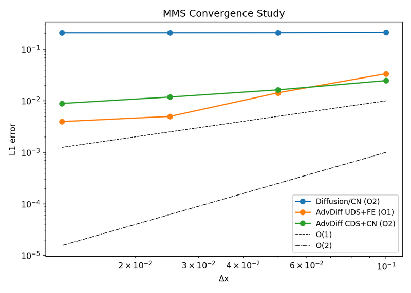
Numerics are checked independently of any specific physics case: a method-of-manufactured-solutions study confirms discretization error shrinks at the theoretically predicted rate under mesh refinement (not just “looks right” on one grid); a von Neumann stability analysis gives the analytical amplification factor for each scheme/time-integrator pairing, cross-checked against the empirically measured stability regions and a CFL-number sweep.

The geometry kernel’s own validation is cross-engine agreement, not just “did it run”: all three independent geometry backends (Gmsh, SDF, PicoGK-compatible) report identical enclosed volume, validity and watertightness for the same test shapes — for example, the revolved-nozzle case, all three engines compute 5.4633×10⁻⁵ m³, valid and watertight.

Two smaller physics studies from the pre-release planning archive round out the picture: a spherical-droplet extinction sweep reproduces the classic U-shaped extinction curve — kinetic extinction at small droplet diameter, radiative extinction at large diameter, with a stable burning window in between (d₀ ∈ [0.20, 3.0] mm in this sweep) — confirming both extinction branches are physically present, not just one. A 2D volume-of-fluid tank-slosh case measures the free-oscillation natural frequency at 5.3235 rad/s against an analytic 5.3156 rad/s (0.15% error), and confirms resonant forcing produces a larger steady-state amplitude than off-resonant forcing, as it must.

The documentation deliberately marks known gaps (no compressible density-based solver, no AMR, no radiation) rather than overstating maturity — that candor is itself part of the engineering discipline here.

Microfluidics validation dossier

The particle-separation application that motivated the whole project gets its own standing validation dossier, not just a demo screenshot: the base 3D pipe-flow field checked to machine precision against the exact Hagen-Poiseuille profile, then a real 3D particle tracer built on that field reproducing the Segre-Silberberg (1962) tubular-pinch mechanism directly — four tracked particles genuinely migrating toward an intermediate equilibrium radius from both directions, not assumed. Curved-duct Dean secondary flow is checked quantitatively against both the low-De (Dean 1928) and high-De (Ookawara 2004) scaling laws, and a predicted four-vortex transition that this model’s own probe does not reproduce is kept in as a disclosed, investigated miss rather than dropped.

The topology-optimization formulation gets the same treatment as the physics: a closed-form Brinkman-channel exact solution the penalization method actually solves (residual under 1e-6 relative, ForwardDiff-checked); the Brinkman-penalization approximation cross-checked directly against a genuinely body-fitted mesh of the same geometry, including a real, mesh-refinement-confirmed non-monotonic conditioning effect; a dissipated-power identity closing to FEM discretization error; and — the actual pre-optimization gate — the analytic design-sensitivity gradient overlaid exactly on a central-finite-difference estimate, since a wrong gradient here would silently break every downstream optimization result.

Geometry creator (new: from-scratch feature-tree CAD)

Building on the cross-engine geometry-kernel work above, a newer sub-project pushes the from-scratch signed-distance-field kernel toward genuine CAD-style feature-tree modeling, dependency-free: revolve (a profile swept into a solid of revolution), fillet (smoothly blending two intersecting primitives, not a sharp boolean seam), shell (hollowing a solid to a specified wall thickness), and exact circular sweep (a disk swept into a torus geometrically, not by discretized approximation) are all implemented and verified by rendering each feature and checking it by eye against its expected geometric identity.

My contribution

Developed by me from scratch, including the reacting-flow arc, the microfluidics solver, the geometry kernel work, the stochastic/UQ module, and all three GUIs, on top of the open-source libraries listed above.

Where this is going

A physics solver where every constraint that mattered for the motivating problem is implemented and testable in-house — not a black box whose failure mode has no path to a fix — moving toward native integration of machine-learning terms inside the governing equations, and a fully independent geometry kernel, as the two areas under active development.

Method-of-manufactured-solutions convergenceA method-of-manufactured-solutions convergence study — the numerical error should shrink at the theoretically predicted rate as the mesh is refined, confirming the solver's discretization is implemented correctly rather than just "looking right." Explain CFD and numerical methods
Numerical stability regionsStability regions for the solver's time-integration schemes — the boundary in parameter space where a numerical scheme stops producing bounded solutions, verified against known theory for each scheme implemented. Explain CFD and numerical methods
SDF-kernel revolved nozzleA revolved-nozzle test shape generated by the signed-distance-field geometry engine — one of three independent meshing/CAD backends cross-checked against each other on the same 15 test shapes. Explain Geometry and kernels
Gmsh-kernel revolved nozzle (cross-engine check)The identical revolved-nozzle shape regenerated through the Gmsh backend — compare directly against the SDF-kernel and PicoGK-kernel versions to see that all three independent geometry engines agree. Explain Geometry and kernels
Turbine fluid-structure interaction resultA coupled fluid-structure-interaction simulation of flow around a turbine blade — the structural deformation and the surrounding flow field solved together, not as two separate uncoupled problems. Explain CFD and numerical methods
Conjugate heat transfer validationA conjugate-heat-transfer validation case — heat conduction through a solid coupled to convective heat transfer in the adjacent fluid, solved as one consistent system. Explain CFD and numerical methods
Boiling curve validationA predicted boiling curve (heat flux vs. wall superheat) compared against expected literature behavior — checking the solver's boiling/phase-change model reproduces the correct nucleate-to-film-boiling transition shape. Explain CFD and numerical methods
Hot-spot ignition: a warm patch turning into a self-sustaining flameWhat ignition actually looks like, computed with PANSOPHIA: a small pre-heated patch -- the kind of hot spot a spark or a hot particle leaves behind -- sits in an otherwise cool, fuel-filled space. For a while it just slowly warms (heat trickling in from the surrounding reaction outpaces the heat leaking away); then, at a real, measured tipping point, the reaction runs away with itself, the patch heats sharply, and it settles into a genuine self-sustaining burning kernel that keeps consuming fuel on its own -- the physical definition of ignition, not just "it got hot." Explain Reaction kinetics
Microfluidics outlet-purity heatmapA heatmap from a ~30-cell parameter sweep showing particle-separation purity at the microfluidic device's outlet across different design choices — the result that motivated building this solver in the first place, after a commercial tool's particle-tracing feature failed to work at all. Explain Microfluidics
Particle-separation resolution sweepHow well the microfluidic device separates particles of different sizes, swept across design parameters — the companion figure to the outlet-purity heatmap from the same application study. Explain Microfluidics
Ornstein-Uhlenbeck sample pathsSample paths of an Ornstein-Uhlenbeck stochastic process — part of the solver's stochastic/SDE turbulence module, used for closure-model validation against known analytical statistics. Explain Uncertainty quantification
Von Neumann stability analysisVon Neumann stability analysis of the discretization schemes — the amplification factor of a Fourier error mode as a function of wavenumber, the analytical companion to the empirical stability-region and MMS-convergence checks above. Explain CFD and numerical methods
CFL-number sweepSolution behavior swept across CFL number — how far the time-step size can be pushed before a scheme's stability limit is reached, benchmarked for each integrator the solver implements. Explain CFD and numerical methods
PicoGK-kernel revolved nozzle (third engine)The same revolved-nozzle shape from a third, independent geometry engine (PicoGK). All three backends report the identical enclosed volume for this shape (5.4633e-05, valid and watertight) — cross-engine agreement, not just three renders that happen to look similar. Explain Geometry and kernels
Lid-driven cavity flowThe classical lid-driven cavity benchmark — a standard test case for verifying an incompressible-flow solver reproduces the expected recirculation structure before it's trusted on harder problems. Explain CFD and numerical methods
Flow boiling in a heated channelA flow-boiling case in a heated channel — phase change under forced convection, rather than the pool-boiling curve above, exercising the multiphase model's response to bulk flow. Explain CFD and numerical methods
2D fluid-structure interaction caseA simpler 2D fluid-structure-interaction case, used to isolate and debug the coupling scheme before it's applied to the full 3D turbine case above. Explain CFD and numerical methods
Micromixer demonstration caseA micromixer demonstration case run directly through the solver's own geometry and meshing pipeline — showing the microfluidics module working end-to-end on a self-contained example, independent of the particle-separation application study above. Explain Microfluidics
Variance-reduction comparisonA variance-reduction technique compared against plain Monte Carlo sampling for the same stochastic quantity — the practical payoff of the SDE module beyond just being able to simulate one. Explain Uncertainty quantification
Stochastic sub-grid-scale closureA stochastic sub-grid-scale (SGS) turbulence closure result — where the stochastic module connects back to the solver's turbulence modeling, not just standalone SDE demonstrations. Explain Uncertainty quantification
3D pipe flow vs. exact Hagen-PoiseuilleThe base 3D pipe-flow field the particle tracer below runs on, checked against the exact Hagen-Poiseuille profile: max relative error 2.7e-14, i.e. machine precision, not just a close-looking curve. Explain Microfluidics
Segre-Silberberg tubular pinch — bidirectional migrationA real 3D flow field and a real 3D particle tracer reproduce the Segre-Silberberg (1962) inertial-migration mechanism directly: all four tracked particles move toward an intermediate equilibrium radius, two from inside moving out and two from outside moving in. The model's own self-consistent equilibrium (0.5R) differs from the literature's fitted value (0.6R) — a disclosed, understood quantitative miss (a direct, expected consequence of using a documented literature substitution for a paywalled fitted coefficient), not a hidden one. Explain Microfluidics
Dean secondary-flow intensity scalingMeasured Dean secondary-flow intensity vs. Dean number in a curved channel: local log-log slope 1.99-2.01 at low De matches Dean's (1928) theoretical De^2 scaling almost exactly, declining toward Ookawara's (2004) De^1.63 high-De asymptote — the classic curved-duct secondary-flow signature, reproduced quantitatively. Explain Microfluidics
Four-vortex transition — a disclosed missA documented miss, kept in rather than dropped: the literature predicts a transition from a two-vortex to a four-vortex Dean secondary flow at a critical Dean number (visible as a 1-to-3 jump in an outer-wall-crossing probe). This model's own probe stays at 1 crossing across the full swept range — investigated directly (a perturbed-restart search relaxes back to the same state at machine precision), so this reads as a genuine limitation of the current formulation, not an under-searched parameter. Explain Microfluidics
Brinkman-channel exact solutionThe closed-form Brinkman-channel velocity profile the density-based topology-optimization formulation actually solves, at four penalization strengths: plain Poiseuille flow smoothly deforms into a thin-wall-layer "plug" profile as the penalization parameter grows, with the ODE residual checked below 1e-6 relative (ForwardDiff-verified) at every value. Explain Microfluidics
Brinkman penalization vs. a body-fitted meshCross-checking the Brinkman penalization method (used for topology optimization) against a genuinely body-fitted mesh of the same geometry: leak velocity inside the penalized "solid" region falls monotonically as expected, but the velocity mismatch outside it is non-monotonic in the penalization strength — a real, mesh-resolution-dependent conditioning effect, confirmed (not just observed) by re-running at 4x finer resolution and watching both the minimum-error location and its achievable value shift in the predicted direction. Explain Microfluidics
Dissipated-power identity checkA physical consistency check on the objective functional a topology optimization would minimize: total viscous dissipation computed one way (integrating Phi(u) over the domain) against computed a completely independent way (pressure drop times flow rate) agree to within FEM discretization error (0.08% and 0.18% for the two viscous-term formulations tested). Explain Microfluidics
Analytic design-sensitivity gradient vs. finite differencesThe pre-optimization gate any gradient-based topology optimization depends on: the analytic design-sensitivity gradient overlaid exactly on a central-finite-difference estimate at every design variable, agreeing to about 1e-10 relative at two different step sizes — a wrong gradient here would silently break every downstream optimization result, so it is checked directly rather than assumed. Explain Microfluidics
S9 geometry creator — revolve featureA from-scratch, dependency-free signed-distance-field CAD kernel's revolve feature: a rectangle profile revolved into an annulus, part of a new feature-tree geometry creator (fillet, shell, sweep, pattern) built on the same SDF representation as the cross-engine geometry-kernel work above. Explain Geometry and kernels
S9 geometry creator — fillet featureThe fillet feature blending two intersecting spheres into a single smoothly-rounded solid — a genuine CAD-style feature-tree operation implemented on the SDF kernel, not a boolean union with a sharp seam. Explain Geometry and kernels
S9 geometry creator — shell featureThe shell (hollow-out) feature applied to a sphere at a specified wall thickness — verifying the kernel can produce genuinely thin-walled parts, not just solid primitives and their booleans. Explain Geometry and kernels
S9 geometry creator — circular sweepAn exact circular sweep of a disk profile producing a torus — a geometrically exact construction (not a discretized approximation) exercising the kernel's sweep-feature machinery. Explain Geometry and kernels
2D structural cantilever: deformed mesh and von Mises stress Explain CFD and numerical methods
Mixing-model comparison Explain Uncertainty quantification
Numerical diffusion on a step profile with UDS, CDS, TVD minmod and TVD superbee Explain CFD and numerical methods
SDF kernel: smooth blend of two spheres (implicit-only shape) Explain Geometry and kernels

How to recreate this plot

Watch

A short screen capture of the Math Visualization Studio. Each step is captioned in the clip.

Steps

  1. Open the controls panel
  2. Pick example 2: FTCS heat at r = 0.55
  3. Press Play: the sawtooth grows
  4. Lower the stability number r to 0.4
  5. Press Play again: the profile stays smooth

Code and PDF notes

Free of cost. I approve each request and reply by email.

To request the files, email me at and mention the item id. project-cfdcore