- sciml
- optimization
vZero — A Neural ODE Research Playground
An interactive Neural ODE research environment unifying 44 hand-cloned training-script versions, with a live FastAPI+React GUI, a widened optimizer zoo, RL-as-a-trainer, symbolic regression, PINN benchmarks, and an executed d2l-style curriculum
datasheet // neural-ode-playground
- images
- 22
- videos
- 0
- formats
- png
- text
- 2596 words · 12 min read
- studio
- /solver?tab=ode&preset=4
- source
- previous site
- topics
-
- optimizer race ×1
- ablation ×1
- rl arena ×5
- dataset geometry ×3
- rl evaluation ×3
- curriculum ×7
- loss and training ×2
On this page0%
Course notes: the mathematics behind this project is written up as a self-built Neural ODE course, with a verified animation for every session.
Problem
sweep/, sweep_normalization/ and sweep_temp/ had 44 hand-cloned copies of essentially the same H2/O2 autoignition Neural ODE training script between the three of them (52 counting a handful of earlier one-off folders) — each one a small, undocumented fork exploring one axis (a different normalizer, a different time-rescaling, a different loss space) with no shared code and no record of which combination did what. Reproducing an old result meant re-reading a specific version’s diff by hand. This project is that: one codebase, one Config object standing in for every version, plus a live, browser-based environment for running and comparing new ones — closer in spirit to TensorFlow Playground and ConvNetJS than to a one-off research script.
Approach
- One
Config, every axis. A single frozen dataclass (config.py) is the entire specification surface — normalizer, loss space/kind, solver, optimizer, architecture — validated on every use so an invalid combination fails at construction time, not partway through a training run. All 44 original versions round-trip through it as presets, verified bit-identical against the real on-disk data and gradients (tests/test_gradient_equivalence.py, exactnp.array_equal). - A live playground GUI. FastAPI backend + React/D3 frontend: pick a preset, override any field, launch a real training run, and watch loss curves, gradient-flow, and value-flow diagrams update over a WebSocket while it trains — one OS process per run, not a thread, so a live run never blocks the server.
- A widened optimizer and objective zoo. From the original 3 gradient optimizers to 11 (SGD through L-BFGS), plus 7 gradient-free backends (CMA-ES, genetic algorithms, Bayesian optimization) driving the same training loop with zero
torch.backward()calls — which unblocks directly optimizing 22 re-implemented fairness/robustness objectives from the MUQ-SAC uncertainty-quantification literature that have no gradient at all. - Architecture as a set of composable slots, not a fixed network. A custom decoder head, a hard mass-conservation constraint on the predicted state, and a dependency-free graph-convolution front layer built over the real reaction-coupling structure of the Cantera mechanism — every slot defaults to the original architecture exactly, verified byte-identical.
- A peer model family that isn’t a neural network at all. PySR symbolic regression, sharing the same data/loss pipeline as the Neural ODE path, so a discovered closed-form right-hand side is directly comparable to a learned network’s test loss.
- PINN benchmarks, method-of-lines style — all four of Raissi’s, plus a CFD classic. A PDE semi-discretized in space becomes an ODE state that fits the existing trajectory machinery exactly: viscous Burgers, Allen-Cahn, KdV, and the nonlinear Schrödinger equation (the genuinely complex-valued one, encoded as real channel pairs with mass conservation verified to 1e-4) — each scored against a real DeepXDE physics-informed-neural-network baseline on the same fine-grid reference solution, with Raissi’s inverse Navier-Stokes benchmark honestly substituted by the lid-driven cavity (Ghia et al. 1982, the standard forward CFD validation case — its converged primary-vortex core matched the paper’s own published location). Real numbers at matched, bounded budgets: Burgers 0.126 (Neural-ODE-MoL) vs. 0.439 (PINN); KdV 0.358 vs. 0.457; Schrödinger 1.186 vs. 1.156 — reported as-is, including the benchmark neither side fits well at this compute.
- An executed, not exported, curriculum. d2l.ai’s optimization and gradient-flow curriculum, run for real against this codebase’s own 12-optimizer registry and gradient instrumentation, rendered directly inside the playground’s own Learn view (not only exported as a download) — every figure in the gallery’s curriculum group is a notebook cell actually executed against this project’s own code, covering gradient stability, vanishing/exploding gradients in shallow vs. deep networks, the model’s literal input-feature representation, and what continuous depth costs relative to discrete layers on a shared classification task.
- An open plugin registry, not a closed enum. Drop a
.pyfile defining a custom activation, regularizer, gradient transform, ODE-solver time-reparameterization, a whole hidden-layer architecture block (a residual layer, say), or a new normalization scheme; it’s auto-discovered at startup and shows up in the GUI’s own dropdowns next to the built-ins — the same schema-derives-from-the-real-registry discipline the optimizer list already used, extended to let a user add to it without touching this codebase. -
Reinforcement learning as a third training strategy, alongside the gradient path and the gradient-free black-box search: a PPO policy (Stable-Baselines3) that treats the loss landscape itself as the environment and a bounded weight perturbation as the action — reachable from the same GUI form as every other training mode, not a separate tool. Session 11: a live RL Arena view closes the last ConvNetJS gap this project had (
rldemo.html’s interactive agent canvas) — the real PPO agent’s actual weight-space trajectory, projected onto a fixed 2D slice (Li et al. 2018’s loss-landscape-visualization technique), with a trailing path and a live action arrow. Beside it, a from-scratch tabular Q-learning PuckWorld (therldemo.htmlpedagogical spirit, re-implemented as a simpler algorithm than ConvNetJS’s own small deep-Q-network — same problem, stated honestly; the RL Arena screenshot lives in the gallery above): - Multi-objective, topology, geometry, and CFD optimization — the user’s own extension. From-scratch NSGA-II (non-dominated sorting + crowding distance, re-implemented from the published formulas, not wrapped from a library), hypervolume and three scalarizations; SIMP topology optimization (verified against known truss patterns) plus a neural-reparameterization variant; and CST airfoil parameterization driving a from-scratch Weissinger vortex-lattice lift solver — validated against thin-airfoil theory’s closed form (0.13% agreement) before being trusted for genuinely-cambered sections — racing a real NSGA-II drag-vs-lift Pareto front. All three reachable as real playground views (Pareto, airfoil) and live-tested
POST /moo/*endpoints, not library calls. - Neural-operator baselines (DeepONet and a Fourier Neural Operator), from scratch. The operator-learning counterpart to the PINN rows: a branch/trunk DeepONet and a 2D spectral-convolution FNO re-implemented from the papers, trained on the same Burgers trajectories the Neural-ODE side uses and scored by the same fine-grid L2 metric — FNO 0.188, DeepONet 0.401 at a bounded 200-epoch first pass, next to PINN 0.439 and Neural-ODE-MoL 0.126 (the FNO’s grid-agnostic spectral layers are what let it evaluate directly at the 8× finer reference resolution). First-pass numbers, no hyperparameter tuning, stated as such.
- A five-view instrument shell, not one long scrolling form: a working Instrument view (edit the network, watch the decision surface and flow field update live, before you even press Run), a narrated Atlas of every visualization technique, a Lab for optimizer races/hyperparameter search/config exports, the Learn curriculum, and a Data view with a real pre-processing pipeline (channel selection, rescaling, resampling, outlier clipping, live before/after) over whatever dataset is currently loaded.
- A public build with zero server dependency. The classification/regression toy-dataset half of the playground — datasets, feature picker, network editor, decision surface — re-runs entirely client-side: a from-scratch multi-layer perceptron (own initialization, own hand-derived backpropagation) trained with
requestAnimationFrame, verified to clear the same accuracy bar as the real PyTorch path on the same problems, not to match it bit-for-bit. Reuses the exact same visualization components as the local app; only the training loop underneath is swapped out. Live at /playground/. - A scroll-driven explainer for people who’ve never seen a Neural ODE. Four live-canvas beats — a vector field, discrete layers dissolving into continuous depth, a real network training in front of you, and this project’s own dynamic-range finding (below) made visible — replacing a static onboarding modal as the playground’s first-visit landing page.
Results
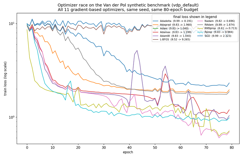
The optimizer race above is one representative real result, not a curated highlight: all 11 gradient optimizers in the registry trained from scratch on the same tiny synthetic problem (a Van der Pol oscillator, this project’s non-chemistry test family), same seed, same budget, re-run for this page with every curve’s real final loss value in the legend. Nadam reached the lowest final loss (0.696); L-BFGS barely moved off its starting point (9.52 → 9.27, effectively stuck) and Adadelta was similarly poor (8.19), both roughly an order of magnitude worse than the best performers on this particular problem — reported as-is, including the optimizers that didn’t do well here. Adam and AdamW land on nearly identical final losses (1.040 vs. 1.040) — a real result of this problem’s small weight-decay setting, not a plotting artifact. This chart covers gradient-based methods only; a genuine heuristic-vs-gradient comparison, with a real genetic algorithm alongside CMA-ES under the same shared-budget discipline, is on the dokimazo project page.
A gradient-free CMA-ES run, driven entirely through the black-box Trainer interface with zero .backward() calls anywhere, reduced a fairness-weighted residual objective from 108,204 to 6,410 over 612 evaluations — beating an equal-budget Adam/MSE run’s own report on the same metric (7,385). On the PINN-vs-Neural-ODE comparison, at matched (session-time-bounded) training budgets, the method-of-lines Neural ODE reached a tighter L2 fit against a shared fine-grid reference than a from-scratch PINN (0.126 vs. 0.439) — neither fully converged, and that qualification is reported alongside the number rather than left out. The ablation study’s headline figure (the 50-run, 5-seed factorial, published here for the first time in session 11: normalizing temperature cuts test loss by roughly an order of magnitude, 2.314×10⁵ → 2.662×10⁴, p = 3×10-15 — normalizing species alone, with temperature left raw, changes nothing, bit-for-bit, because temperature’s gradient already owns effectively 100% of an equal-weight loss) lives in the gallery above.
The flow-field view above (the demo embedded on the home page) is the newest of these: a Neural ODE’s learned right-hand side dy/dt = f(y) genuinely is a vector field, so the playground animates it directly — particles advecting through the model’s own learned dynamics, with the known true right-hand side overlaid whenever one exists (the Van der Pol system, μ=1). On a short, bounded training run, the learned-vs-true RMS error over that field measurably shrinks with training, checked directly rather than assumed — the concrete claim the feature makes, not just “the picture looks reasonable.”
Benchmark case studies
Every physics benchmark this project runs is reported here as its own case study — the same discipline as the ablation result above: real numbers, matched bounded budgets, and the bad ones published too. “PINN” is a from-scratch DeepXDE physics-informed neural network (collocation-point residual minimization, run as an independent subprocess); “Neural ODE (MoL)” is this project’s own method-of-lines Neural ODE trained through the regular playground loop; both are scored by the same L2 relative error against a shared fine-grid reference solution, so the numbers are directly comparable. None of these are fully-converged, publication-grade fits — each row’s budget is stated, and that qualification belongs to the number, not to a footnote.
| Case study | Physics | PINN (L2 error) | Neural ODE, MoL (L2 error) | Read of the result |
|---|---|---|---|---|
| Burgers (Raissi, viscous, ν=0.01/π) | shock-forming nonlinear transport | 0.439 (1000 Adam iters) | 0.126 (400 epochs) | The first benchmark (2026-08-24): at equal session-time budget the method-of-lines Neural ODE fits noticeably tighter |
| Allen-Cahn (periodic, stiff bistable reaction) | interface/phase-field dynamics | 0.993 (3000 Adam iters) | 0.032 (800 epochs) | The widest gap of the set: the stiff reaction term is the part a collocation-point PINN struggles with at this budget |
| KdV (third-order dispersive, solitons) | nondissipative wave dynamics | 0.457 (3000 Adam iters) | 0.358 (800 epochs) | Closest race: MoL slightly better; the PDE residual still sees the true third derivative on the PINN side despite a DeepXDE PeriodicBC order-2 limitation, stated not hidden |
| Nonlinear Schrödinger (complex-valued, soliton) | quantum/optics envelope dynamics | 1.156 (3000 Adam iters) | 1.186 (800 epochs) | Genuinely hard for BOTH at this compute budget — published as-is, including the row where this project’s own side loses |
| Lid-driven cavity (Ghia et al. 1982, Re=100) | steady incompressible recirculation | — (no PINN baseline; scoped out, stated in-code) | validated, not just run: the converged streamfunction’s primary-vortex core landed at (x≈0.67, y≈0.80) vs. the paper’s own published (0.62, 0.74) | Raissi’s inverse cylinder-wake Navier-Stokes benchmark has no clean forward method-of-lines analogue; the standard forward CFD validation case was substituted explicitly, not silently |
Neural-operator baselines (session 12), same scoreboard: on the Burgers case study, a from-scratch DeepONet reaches 0.401 and a 2D Fourier Neural Operator reaches 0.188 at a bounded 200-epoch first pass (no hyperparameter tuning, stated as such) — the FNO lands between the PINN and the Neural ODE, and is the only row evaluated at the fine 512-point reference grid without retraining (spectral layers are grid-agnostic; zero-shot resolution transfer is the technique’s defining property).
RL-as-trainer: a declared-criteria-first evaluation
Rather than judge the PPO trainer by whether its loss curve “looks reasonable,” a later evaluation pass declared its pass/fail criterion before reading any result: RL adopted only if its best objective value, at a matched evaluation budget, comes within 2x of the better of this project’s own CMA-ES and Nelder-Mead backends on the same problem, run through the identical objective-function seam so no backend gets an unfair shortcut. The measured outcome — RL at 1.09x the better comparison backend — clears that bar, and the verdict card states its own scope plainly: a first-pass PPO implementation vs. this project’s own two gradient-free backends, on one synthetic problem, not a general claim about RL versus optimization. Every number on the verdict card is generated directly from the run, never hand-typed.
This is the same discipline the ablation study above and the broader H2/O2 architecture campaign both use — criteria fixed first, real numbers reported whichever way they land — applied here to the playground’s own RL trainer rather than to the withheld chemistry-architecture research.
Dataset geometry: what the split actually tests
Before trusting any accuracy number from a train/validation/test split, two questions have to be answered directly rather than assumed: does the test set sit inside the training distribution (interpolation) or outside it (extrapolation), and how different do the underlying trajectories actually look across species with wildly different dynamic range? The gallery’s dataset-geometry group answers both: a 2D split-geometry check confirms every held-out point of the random-pool preset sits inside the training convex hull (a genuine interpolation test), while a second, deliberately structured preset places interpolation and extrapolation test points on opposite sides of the training grid on purpose, so the two failure modes can be told apart. A trajectory-bundle figure overlays every split’s own T, H2O, OH and HO2 trajectories directly — the eight-decades-of-dynamic-range problem the entire normalization ablation above exists to address, made visible rather than only reported as a number.
The optimizer-race notebook, executed
The notebook behind the figure above, embedded in full — every cell was run for real (headlessly, via nbclient) against this project’s own code, not hand-typed:
Validation
Every refactor is checked against four bit-identity gates before being considered done: exact forward-pass equality (rtol=0, atol=0) and exact gradient equality (np.array_equal) against the real, pre-existing training data, plus a check that turning instrumentation on or off never perturbs the RNG stream or the numbers it produces. New architecture/optimizer/model-family additions default to the prior exact behavior and are checked against that default before anything new is exercised. The playground’s own backend is tested against a real FastAPI TestClient, including full process-lifecycle tests that spawn an actual training run and follow it over a WebSocket to completion.
My contribution
Sole author of the original 44 training-script versions this project unifies, and of the unification, GUI, and every extension described above.
Where this is going
Held-out gaps, reported rather than hidden: the fairness-objective library’s outlier-robustness clamp is calibrated for chemistry-scale residuals and doesn’t yet rescale correctly for the much larger residual magnitudes a PDE-based problem family produces; the reinforcement-learning trainer ships as a real, tested capability but without ConvNetJS’s own rldemo.html-style live interactive canvas view of an agent stepping; and the pre-processing panel is an exploration tool over an already-generated dataset, not yet a way to commit a chosen pipeline back into a real training run. None of these are silently worked around — each is a stated, scoped-out follow-up.
Gallery
How to recreate this plot
Watch
Steps
- Open the controls panel
- Pick example 1: A saddle
- Type probe x = -1.2
- Type probe y = 0.9
- Raise the contour lines to 28
Code and PDF notes
Free of cost. I approve each request and reply by email.
To request the files, email me at krunalpanchal1995 [at] gmail [dot] com and mention the item id. project-neural-ode-playground