- optimization
- sciml
dokimazo — A PIDO Optimization Workbench
A dependency-light process-integration-and-design-optimization workbench with a plug-and-play graph IR, closed by a reinforcement-learning conformer search that tunes a long alkane chain's rotors one at a time
datasheet // dokimazo
- images
- 12
- videos
- 9
- formats
- png, mp4
- text
- 3523 words · 17 min read
- studio
- /mechanism?preset=19
- source
- previous site
- topics
-
- rl rotor search ×4
- solver visualization ×8
- uncertainty propagation ×1
- identity vine mark ×2
- topology optimization study ×2
- identity refining fire ×2
- third party connector ×1
- aircraft design ×1
On this page0%
Problem
Commercial optimization/design-of-experiments packages (Ansys, COMSOL, Mathematica, MATLAB) bundle objective functions, algorithms, and data handling into one fixed pipeline — swapping any one piece usually means switching packages entirely, or writing glue code that itself becomes unmaintainable. The everyday optimization problems across chemistry, ML training, and design search share the same shape (a decision vector, an objective, a search strategy) but never share a codebase: a conformer search, a neural-network training run, and a multi-objective engineering design each get re-implemented from scratch, with no common graph to mix and match objectives, solvers, and samplers.
dokimazo is a from-scratch answer: a numpy-only core (a graph intermediate representation where objective functions, solvers, adapters, samplers, and NN trainers are all swappable, lazily-discovered plugins) with every heavier capability — jax-backed neural-network training, RDKit-backed chemistry, a browser GUI — kept strictly optional and outside the kernel.
Approach
- A minimal, protocol-driven kernel. Four parallel
Registrygroups (Solver,Adapter,Trainer,Sampler) share one lazy-discovery mechanism — entry points or explicit in-process registration — so a new algorithm plugs in without touching the kernel.Problem(a DESDEO-flavored decision-vector/objective/constraint container) and a content-addressedGraph/NodeIR are the only two things every capability composes over. - Six solvers, cross-checked against each other. Three clean-room native implementations (Nelder-Mead, IPOP-CMA-ES following Hansen 2001/2016 and Auger & Hansen 2005, L-BFGS-B) plus thin, tested wrappers around
scipy.optimize,pymoo,pygad, andoptuna— every one benchmarked head-to-head on a shared analytic/engineering/multi-objective suite (Dolan–Moré performance profiles, hypervolume/IGD indicators). - Sampling, uncertainty propagation, and solution mapping as first-class graph nodes: Monte Carlo and QMC (Sobol′/Latin-Hypercube) samplers, forward uncertainty propagation, and Pareto-front solution mapping via fast-non-dominated-sort (Deb et al. 2002).
- A jax-backed NN/training layer — one
Trainerprotocol covering supervised and RL losses identically (a REINFORCE loss and a supervised loss are the same shape to the trainer that minimizes them), with a hard-boundary-condition decoder (Lagaris et al. 1998), a graph-convolution layer (Kipf & Welling 2017), a hand-rolled fixed-step Neural ODE (Chen et al. 2018), and REINFORCE (Williams 1992) as four ways of building that one loss. - A browser GUI, built the same session a plan mistakenly called it “explicitly parked” and the user pointed out that had been the actual request — a FastAPI backend plus a dependency-free vanilla-JS node-graph editor: draw the pipeline, wire nodes by clicking output-then-input dots, run it, and watch dependency-free inline-SVG charts (histograms, Pareto scatters) render from whatever shape the run’s output takes.
- Reinforcement learning closing its own named gap, on a real application — this project’s newest piece. Every capability above ships with its fidelity gaps named in its own docstring rather than silently rounded up (
REINFORCE on a single-step contextual banditwas RL’s own stated gap). Closing that gap with a second toy bandit would have been easy; instead it’s closed with an RL agent that tunes the rotatable bonds of a real molecule — n-dodecane, a 12-carbon chain — one rotor at a time, searching for the conformer (3D shape) with the lowest MMFF94 force-field energy. See the training curve and benchmark figures above.
The RL rotor-tuning environment
A RotorTuningEnv episode is one left-to-right pass over the molecule’s 11 rotatable backbone bonds: at each step the agent picks a discretized angle (24 bins, 15° resolution) for the next rotor, conditioned on every rotor already set. Two measurements, taken directly on this machine before writing a line of the reward design, decided its shape:
- A full relaxed MMFF94 energy evaluation (
Minimize()+CalcEnergy()) costs 14.7 ms. - The same energy without relaxation — a single-point evaluation — costs 0.26 ms: roughly 56× cheaper.
That asymmetry is why the reward is split in two: every step pays the cheap single-point energy improvement as a dense shaping signal, and only the final step — once every rotor is decided — pays for one real, relaxed energy evaluation as the terminal reward, which is the number that actually gets reported. The policy is trained with multi-step REINFORCE (Williams 1992): discounted reward-to-go plus a per-timestep batch-mean baseline for variance reduction, extending — not replacing — this project’s existing single-step REINFORCE loss.
One invariant is load-bearing enough to be checked by its own test: the environment holds no mutable geometry between steps. Its entire state is the plain vector of angles chosen so far; every reward call resets to a fixed reference geometry and sets the full vector from scratch. An earlier version of this project’s own conformer-energy function once violated exactly this rule by accident — mutating a molecule’s 3D coordinates in place with no reset, so the same input silently returned two different energies — which is precisely the kind of bug that breaks a content-addressed cache. The new environment is built so that class of bug can’t recur, and a regression test replays the same episode twice (and interleaved with an unrelated one) to confirm it.
Results
n-Dodecane, not this project’s earlier conformer-search molecule, is the headline case specifically because it has an independent ground truth: the global MMFF94 minimum of any unbranched alkane is its all-anti extended conformer — every backbone torsion at ±180° — a structural fact, not an agreement between two implementations. (The earlier flagship result, on a smaller molecule whose SMILES reading was never confirmed with the user, stays out of this page for exactly that reason.)
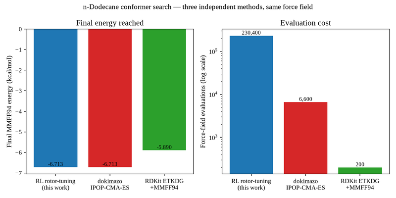
Three independent methods, same molecule, same force field, reported side by side whether or not the new one wins:
| Method | Final MMFF94 energy | Force-field evaluations | Wall time |
|---|---|---|---|
| RL rotor-tuning (this work) | −6.7129 kcal/mol | 230,400 | 14.7 min |
| dokimazo’s IPOP-CMA-ES | −6.7129 kcal/mol | 6,600 | 1.5 min |
| RDKit ETKDG + MMFF94 (200 confs) | −5.8895 kcal/mol | 200 | 5.3 s |
Both the RL agent and IPOP-CMA-ES reached the true global minimum — verified directly, not inferred from the energy number alone: reading back the molecule’s actual post-relaxation dihedral angles (not the pre-relaxation guess a solver proposes — MMFF94’s own geometry relaxation moves torsions too, so those two are genuinely different things) shows all 9 real backbone C–C–C–C torsions sitting within numerical precision of the all-anti ±180° target, matching a directly-computed all-180° reference energy (−6.712879 kcal/mol) to 6 significant figures. The other 2 of the 11 bonds RDKit’s rotatable-bond detector flags are dihedrals through a terminal methyl group’s own hydrogens — rotating one changes the energy not at all (checked directly: bit-identical energy from −60° to 180°), since permuting three symmetric hydrogens isn’t a real conformational degree of freedom. RDKit’s own 200-conformer ETKDG reference, by contrast, landed on a genuine local minimum 0.82 kcal/mol above the true global one — the honest way this project’s earlier conformer-search result put it still applies here, just with the roles reversed: this time, the harder-to-reach oracle (structural ground truth) is what dokimazo’s own search reached and the standard reference pipeline missed, at roughly 35× (CMA-ES) to 1,150× (RL) more force-field evaluations to get there. The RL agent’s own post-relaxation dihedrals were not independently re-extracted (would need re-running its ~15-minute training) — its evidence is the energy value matching CMA-ES’s and the direct reference’s to displayed precision on a continuous, 11-dimensional, non-convex function, which is itself strong, but that is what it is: an energy match, not a separately re-verified geometry, and that distinction is worth keeping straight rather than blurring the two kinds of evidence together.
The training-curve figure above shows the RL agent’s batch-mean and best-so-far energy over 400 REINFORCE training steps against both reference methods as horizontal lines — the best-so-far curve reaches CMA-ES’s exact value by step ~30 and holds it for the rest of training, while the batch mean keeps improving as the policy gets more consistent at finding it. The torsion-convergence figure shows the 11 raw rotor-angle proposals (including the two degenerate methyl ones, since it’s tracking what the agent actually proposed) over the same training run. The video is the same optimization process, rendered as the molecule’s real 3D structure at each improving checkpoint.
Solver, sampler, and solution-mapping visualization
The Approach section above names six cross-checked solvers, quasi-Monte-Carlo sampling, and Pareto-front solution mapping as capabilities — the gallery’s “solver visualization” group is the first time any of that is shown rather than just described, built with a small new instrumentation layer (dokimazo.viz) that wraps a real Solver.minimize call and records every evaluation against a shared cumulative-function-evaluation clock, not iteration count (different solvers do very different amounts of work per iteration, so comparing by iteration alone would make a gradient method look free next to a population-based one for no principled reason).
The two solver races make the same point two different ways, now across five solvers — two gradient-based (dokimazo’s own L-BFGS-B and an independent SciPy L-BFGS-B reference), one derivative-free point-iterate method (Nelder–Mead), and two population-based heuristics (CMA-ES, an evolution strategy, and a genetic algorithm via PyGAD) — every legend entry naming both the algorithm and which family it belongs to, and every race’s own poster figure carrying a final speed/accuracy scoreboard (each solver’s ending loss value next to its evaluation count) so the comparison doesn’t require reading the plot by eye.
On Rosenbrock’s single smooth valley, both L-BFGS-B implementations and Nelder–Mead all reach machine precision (f < 6e-18) in 200-240 evaluations; CMA-ES gets there too but needs roughly 10x the budget (2,300 evaluations) to do it, and the genetic algorithm — genuinely the heuristic comparison this figure was missing — spends more than double CMA-ES’s budget (4,685 evaluations) to land at f ≈ 0.025, close but not machine-precision. Rastrigin’s many local minima tell a different and genuinely more interesting story than a smooth valley can: this run, both L-BFGS-B implementations happen to reach the true global optimum directly (f < 2e-14, in as few as 11 evaluations) rather than stalling nearby, CMA-ES also reaches it (in 1,592 evaluations), while Nelder–Mead (f ≈ 31.8) and the genetic algorithm (f ≈ 0.56) both get stuck in local minima on the same shared budget — a reminder that “gradient methods get trapped on a multimodal function” is a tendency, not a law, and this is what actually happened on this run, not what the setup was expected to show.
The trajectory figure is this page’s literal answer to “a 3D surface trace for a three-variable system”: a height-map surface (z = f(x, y)) only exists for exactly 2 inputs and 1 output, so for a genuine 3-decision-variable problem the mathematically honest visualization is every evaluated point plotted at its own (x1, x2, x3) coordinate, colored by objective value, with the converging search path traced through that space rather than a surface mislabeled as one.
The sampler and solution-mapping figures are each an honest demonstration of one specific capability, not a cherry-picked result: quasi-Monte-Carlo’s more even coverage is shown both visually and via its actual discrepancy number against plain Monte Carlo, and the extracted Pareto front is captioned for what it does and doesn’t show — it correctly extracts the non-dominated subset of whatever sample it’s given, but a sample built by plain random search sits visibly above the true front, which is a fact about the sampling, not the extraction, and the honest reason a real multi-objective solver (open roadmap item, see below) is a different, still-needed piece.
For the two-variable case a height-map surface is the honest visualization the trajectory figure above deliberately avoids for three variables: two fixed-camera surfaces (Rosenbrock’s single curved valley, and Himmelblau’s four separate equal-depth basins) each animate a real CMA-ES run’s full evaluation cloud and best-so-far point walking from its initial guess to the minimum, in true evaluation order, with a synchronized panel tracking that same run’s objective value actually dropping (log scale) as the search converges — the point moving is the search converging, not a camera sweeping around an already-finished answer — with a companion fixed-slice figure showing exactly how that changes once a third variable is added — the (x1, x2) path from the earlier 3-variable trajectory result, projected onto a 2D slice held at the run’s own found x3, with the figure’s own title stating plainly that the slice height and each point’s true 3D objective are different quantities. Forward uncertainty propagation gets the same “just another graph node” treatment as sampling and solution mapping: Monte Carlo propagation of Normal input uncertainty through Rosenbrock, mean and ±1σ read directly off the output histogram.
Validation
Every algorithm in this package is oracle-tested against an independent reference before being trusted, never “it looks right”: the native solvers against scipy’s own convergence on the same analytic functions; MMFF94 energies against RDKit’s own force-field implementation (the same numbers, since dokimazo calls RDKit’s force field directly — the search strategy is what’s independent, not the physics); the RL rotor-tuning environment’s purity against a bit-for-bit replay test; and the REINFORCE loss (both the original single-step version and this session’s multi-step generalization) against a synthetic environment with a known-optimal action, checked directly rather than by “reward went up.” The full test suite has grown to 369 passing (1 skipped by design) as the package picked up its browser GUI and benchmark harness — up from 184 at the time of the RL rotor-tuning result above.
A standing benchmark harness now cross-checks 7 solvers (including two independent L-BFGS-B implementations) across 16 analytic problems plus a constrained-engineering suite, reporting Dolan–Moré performance profiles rather than a single leaderboard number — a losing row is kept in the table exactly as visibly as a winning one, the same discipline as the RL-vs-CMA-ES-vs-RDKit table above.
My contribution
Sole author of the kernel, every solver/sampler/trainer/adapter, the web GUI, and the RL rotor-tuning environment and loss described above — a personal, from-scratch package, built and cited against the published algorithms it reimplements (Hansen, Williams, Halgren, Deb et al., Kipf & Welling, Chen et al., Lagaris et al.), not a wrapper around them.
Physical geometry optimization, third-party connectors, and gradient vs. heuristics
The RL result above closed a gap in dokimazo’s chemistry application; this later session closed a different, longer-standing gap — nothing in the package optimized a physical shape subject to real physics, and nothing proved the package’s “plug in any third-party code” claim on an actual external solver rather than a toy subprocess.
Third-party connector kernel. dokimazo.objectives.external (a sixth objective source, alongside the typed-expression/benchmark/Python-file/command/HTTP ones already built) is what an expensive external solver needs that a cheap disposable subprocess doesn’t: a persistent, content-addressed case directory (dokimazo.exec.cases.CaseStore) instead of a vanished temp dir, a disk-backed evaluation cache, and — the one addition that actually separates a toy connector from a usable one — a configurable failure policy (raise/penalty/inf) plus retries, since a real CFD/kinetics solver diverges on some fraction of proposed design points as a matter of course, and today’s toy connector would simply abort the whole search on the first one.
Proven on two real, independent physics codes from PANSOPHIA, this author’s own from-scratch CFD/combustion package, treated genuinely as a black box — no dokimazo kernel change to add either, only a driver script on the shared params.json → result.json contract:
- Rocket-nozzle shape optimization through PANSOPHIA’s real quasi-1D Euler CFD solver (
solve_quasi1d_euler): two design variables (throat position, exit/throat area ratio), Nelder-Mead, 37 real external-process CFD evaluations (~9s each — Julia’s own interpreter/JIT cost, measured directly before designing the budget around it, dominates the actual ~0.2–0.8s physics solve). Nozzle thrust improved from 4.328e6 to 4.367e6 N-equivalent. - “Refining fire” (1 Peter 1:7) — see the Identity section below — a genuinely constrained combustion optimization through PANSOPHIA’s real 36-species GRI-Mech 3.0 kinetics (
ignition_delay/StiffReactor), exercisingdokimazo.constraints.PenaltyContinuationfor real rather than only box bounds.
A formulation tried and rejected, reported honestly rather than hidden: the original plan for the fire case used PANSOPHIA’s freely-propagating 1-D laminar flame solver. Checked directly before committing to it — this package’s own standing discipline, never “it looks right” — its measured flame speed came back bit-identical across genuinely different design points at a mesh coarse enough to fit an optimizer’s budget: a real mesh-resolution degeneracy, not something honestly optimizable. The stiff-reactor ignition-delay formulation replaced it, confirmed non-degenerate the same direct way before any optimization code was written around it.
Gradient vs. heuristics, on a problem large enough for the gap to be real. The user’s own ask — show where gradient-based search wins and RL/GA genuinely fail — needed a problem with an available exact gradient a heuristic structurally cannot use, so this runs entirely in-process: SIMP compliance-minimization topology optimization (dokimazo.physics.topopt, new 2-D plane-stress FEA kernel, Bendsøe & Sigmund), self-adjoint by construction — an exact gradient costs one extra element-local vector operation, no second linear solve. At 288 correlated design variables, an equal ~150-evaluation budget, and — critically — the same exact volume-constraint projection applied to every arm (so no arm can fail for worse constraint handling rather than lacking a gradient): Optimality-Criteria descent reaches compliance=143.7; PyGAD’s genetic algorithm reaches 593.3 while actually using roughly double the evaluation budget (303 evaluations — a stronger result for the gradient method, not a weaker one, reported as measured rather than forced to match); a REINFORCE policy over a new static-Gaussian action space (Williams 1992’s own continuous-action derivation, extended here) reaches 577.1. Gradient wins by ~4x over both. The gap this closed while building the REINFORCE loss is itself a small case study in this package’s own verification discipline: an earlier version silently carried zero gradient with respect to the policy mean (it reused independent sampling noise directly in the log-probability term instead of the fixed sampled action) — caught by hand-deriving the expected score-function gradient and checking jax.grad against it, not by “training loss went down,” which would not have caught it.
A second gradient-vs-heuristics case, on a real shape problem this time. The SIMP result above is a density field; dokimazo_aero.panel_method extends the same “exact gradient beats a heuristic at equal budget” story to an actual airfoil shape — a jax-native vortex-panel numerical solution of the thin-airfoil boundary-value problem (Anderson’s Fundamentals of Aerodynamics, the discretized counterpart of the closed-form Fourier solution the rest of this pack already used), differentiated exactly through the real linear solve via jax.grad, not a finite-difference approximation. The design space is a free-form sine-series camber line (as many independent shape harmonics as kept, not the fixed 2-parameter NACA family), and at the pack’s own default settings gradient ascent reaches $c_l = 2.265$ in 40 evaluations, while PyGAD’s genetic algorithm — at roughly double that budget (82 evaluations) — only reaches $c_l = 1.821$: the gradient method wins on both quality and cost, the same direction the SIMP comparison found. The video below (a 2-harmonic run, chosen only so the converged shape reads unambiguously as “an airfoil” rather than a higher-harmonic wiggle — a rendering choice, not a different optimizer) opens with a literal rectangular block morphing into the optimizer’s own flat-plate starting point — clearly marked as an illustrative establishing shot, never claimed as solver output — before showing every subsequent frame as a real, unedited gradient-ascent step to the converged cambered shape.
Identity
The package is dedicated to Christ; the cross is already taken by another project in this author’s portfolio (PANSOPHIA), so dokimazo’s own identity comes from two other scriptural images — each expressed as a real optimization result, not drawn, with every human design choice (domain shape, load case, ink color) stated plainly alongside what the solver itself produced (docs/IDENTITY.md in the repo).
“I am the vine, you are the branches” (John 15:5) — the SIMP kernel above, pointed at a domain built specifically to produce branching: a single trunk support carrying a distributed canopy load. Every branch, its thickness, and where it splits is 100% the solver’s own converged density field; the video is real recorded SIMP iterations, not staged frames.
“…tested by fire” (1 Peter 1:7) — the refining-fire optimization above, read literally: the fire must be hot enough to consume the dross without destroying the gold, which is a constrained optimization (minimize ignition delay subject to a temperature ceiling), not a metaphor stretched to fit. The optimizer converged to a final temperature 24.6 K under its 2320 K ceiling — a genuinely binding constraint, not a slack one — and the video is that real reactor’s temperature trajectory climbing to it.
Where this is going
Named, not hidden: the rotor-tuning environment discretizes each angle into 24 bins rather than searching continuously, decides each rotor exactly once in a fixed left-to-right order rather than revisiting earlier choices, and uses only a batch-mean variance-reduction baseline rather than a learned value function. The two new physics connector cases pay Julia’s own per-call startup cost on every evaluation (~9s for the nozzle, ~5–12s for the fire case) — a persistent-worker mode would remove that ceiling but wasn’t built this session, a named deferred capability rather than a silent one. Airfoil geometry optimization (named in the same ask as the nozzle) is no longer deferred — see the jax-native panel-method result above. The broader package still has an open roadmap toward automatic differentiation, a wider deterministic and global-optimization solver suite, full multi-objective algorithms (NSGA-II/III, MOEA/D), Bayesian optimization with surrogate models, global sensitivity analysis, and inverse/calibration uncertainty quantification, plus a stated, honest capability-gap roadmap against Mathematica/MATLAB/EES-class software rather than a claim of parity — this is one growing set of closed gaps on a workbench still being built, not a finished product.