All projects

  • experimental

flamelab

A computer-vision instrument that measures flame length, width and flicker from pool-fire video in physical units with propagated uncertainty — regime classification, cross-run ensemble statistics, and thirteen analysis methods
25 images · 21 videos · 8 min read

flamelab

datasheet // flamelab

images
25
videos
21
formats
png, mp4, gif
text
1617 words · 8 min read
source
previous site
topics
  • campaign ×8
  • fluctuation ×3
  • measurement ×4
  • methods ×2
  • run ×4
  • zonal ×8
  • evaporation ×2
  • boundary validation ×2
  • qc ×2
  • aliasing ×1
  • segmentation ×2
  • kymograph ×1
  • physics ×1
  • dynamics ×3
  • stitching ×3

Agenda

flamelab is a measurement instrument, not a video editor: it turns 4K pool-fire footage into per-frame flame geometry (length, width, tip position) in millimetres with propagated uncertainty, classifies the flame’s dynamical regime through its Hopf-bifurcation sequence, and aggregates repeat experiments into ensemble statistics with defensible error bars. Every number carries units, uncertainty and provenance — and where the footage cannot support a trustworthy number (e.g. a frequency near the camera’s Nyquist limit), the pipeline refuses and says so rather than guessing.

Problem

Combustion dynamics are usually measured with a ruler and a stopwatch — or with diagnostics (laser sheet imaging, chemiluminescence filters, intensified cameras) that a small lab cannot run on every experiment. A consumer 4K camera is cheap, but its footage is hard to quantify honestly: veiling glare inflates the apparent flame boundary, 4:2:0 chroma subsampling and unknown ISP processing corrupt colour-based diagnostics, and the 23.976 fps frame rate aliases the flicker frequencies that matter most. flamelab is built around those exact limits: correct the glare, propagate the segmentation uncertainty, and never report an aliased frequency as if it were physical.

Approach

  • Sub-pixel, glare-corrected contour — veiling-glare correction followed by a multi-gate flame-component selector (brightness, area, rim-anchoring, axis overlap), anchored to the burner rim measured once per video. On the full 13,127-frame reference recording, dropout frames went from 5.1% to 0.0%, and the detected rim agrees with an independent measurement to 0.45 px.
  • Physical quantities with uncertainty — length, width, area, rugosity, tip angle and pinch-off events in mm (ruler-photo calibrated, honesty-flagged as not caliper-confirmed), each with systematic (segmentation) and statistical uncertainty separated.
  • Regime classification — a hidden-Markov classifier over sliding-window spectral features labels every frame with the literature Hopf sequence: Ignition Transient → Steady Laminar → Flickering Onset → Periodic Flickering.
  • Ensemble statistics across repeat runs — eight repeat n-heptane pool-flame recordings (the same experiment repeated), aggregated with bootstrap confidence intervals, ICC variance decomposition, ANOVA/Levene tests, GUM-combined uncertainty, and an ignition-aligned frame matrix.
  • Thirteen analysis methods wired to figures and CSV data — continuous wavelet transform, skeleton/pinch-off precursors, phase-averaged puff-cycle reconstruction, onion-peeling Abel inversion, correlation dimension and largest Lyapunov exponent (each with an explicit reliability flag), Hilbert–Huang/EMD, TV-L1 optical flow cross-checked against kymograph convection velocity, active contours, windowed full-frame POD/DMD, growth-rate fitting at onset, change-point onset detection, and the literature-standard 50%-intermittency height.
  • Zonal seismograph instrument — the same real-time tracked boundary and numeric HUD (height, area, volume, heat-release-rate proxy, tip position), but with the flame split into height zones (McCaffrey’s continuous/intermittent/plume regions among the schemes tested) and a scrolling per-zone width trace, so where a fluctuation originates is visible, not just that it happened.
  • Evaporation/burning-rate physics — a Zukoski-scaled burning-rate proxy fit per run (rise time to 90% of steady rate, growth-scale, overshoot), pooled ignition-aligned across the ensemble.

Implementation

Python with OpenCV, NumPy/SciPy and scikit-image; a ~300-test suite; and three reproducible drivers — one per run (run-analysis.py), one for the cross-run ensemble (run-ensemble.py), and one for the methods (run-methods.py). Outputs are data-first: per-frame HDF5/CSV tables, a CSV next to every figure containing the exact plotted columns, and standalone plotting scripts so any figure can be edited and re-plotted without the pipeline.

Results

The campaign is eight repeat n-heptane pool-flame runs from one recording session. Detection is successful on 96.8–99.8% of frames per run. The headline measurements, with their honesty caveats on record:

  • Ensemble flame height — 110.1 mm (bootstrap 95% CI [75.0, 124.5] across the 8-run campaign; GUM-combined uncertainty ±12.7 mm). Restricting to the three runs with a validated burner-rim anchor gives 117.2 mm [107.9, 123.7] — the two reference-frame definitions are kept separate on purpose.
  • Ensemble width — 16.3 mm [14.6, 18.2] across all runs; 13.7 mm [12.3, 14.4] for the anchored subset (width at one burner diameter above the rim — a different physical quantity than the unanchored fallback, documented, not pooled silently).
  • Run-to-run structure — variance decomposition: ICC 0.42 (height) / 0.52 (width) — real between-run differences exist on top of within-run flicker, and ANOVA confirms the run means differ.
  • Puffing frequency — 0.40 Hz [0.29, 0.52], consistent across all runs, ~35× below the classical pool-fire correlation’s ~13.9 Hz prediction. Two honest candidate explanations are on record: a genuinely different flow regime at this small scale, or aliasing of a true 10–15 Hz oscillation against the 11.99 Hz Nyquist limit. Resolving this needs higher-frame-rate re-acquisition — flagged, not spun.
  • Regime sequence — every run follows the same Ignition → Steady → Flickering Onset → Periodic sequence, with the onset time located to a bootstrap confidence interval per run, and positive oscillation growth rates (0.004–0.047 s⁻¹) across all runs at onset — the supercritical-Hopf signature.

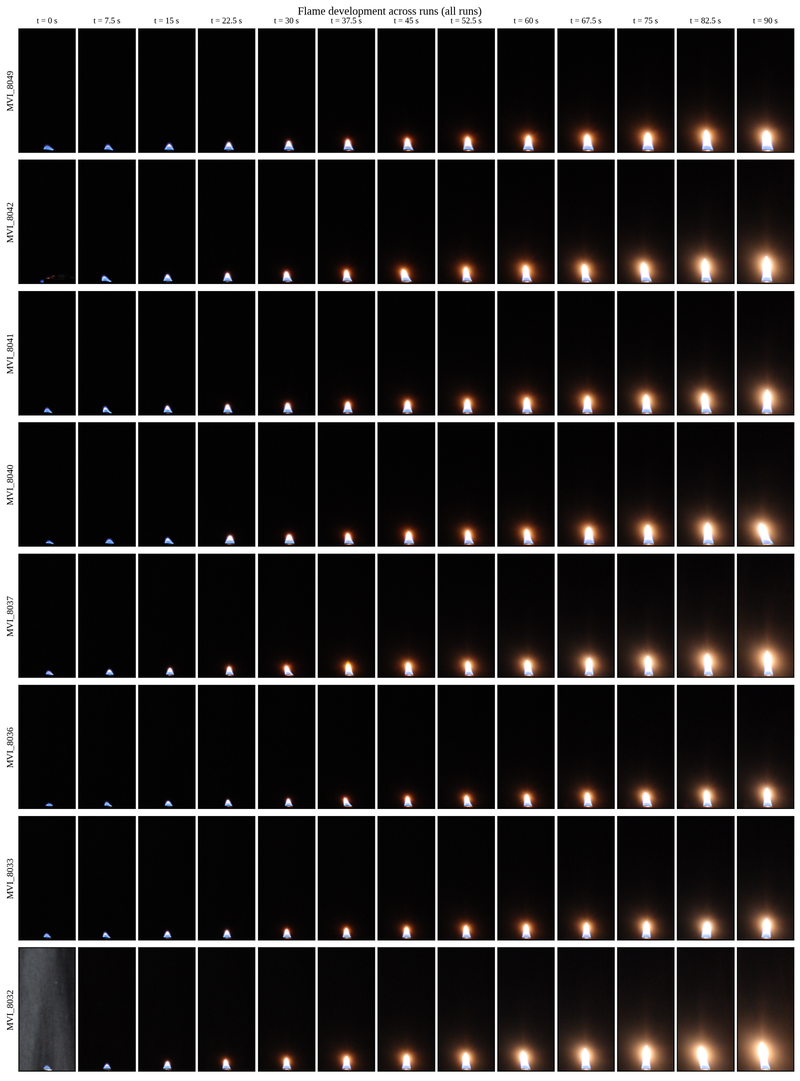
The gallery above shows the ignition-aligned frame matrix (same physical field of view in every cell), the seismograph-style tip and width fluctuation charts, the ensemble traces with uncertainty bands, kymographs, POD/DMD modes, the per-regime overlay videos with the detected contour burned onto the real footage, and the zonal seismograph videos described below. The ensemble power-spectral-density figure is the direct spectral evidence behind the puffing-frequency measurement above, and the per-run flickering-onset-time and anchored-subset-robustness figures make the run-to-run repeatability question directly inspectable rather than folded into one summary statistic. A sample of the live measurement:
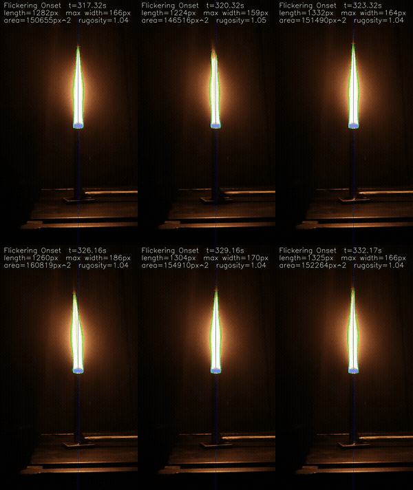
The measured contour, centerline and tip tracking the flame through the flickering-onset transition
The flickering-onset transition with the measurement burned onto the real frames — green: measured boundary, cyan: centerline, red cross: tip, blue: burner axis (full-resolution overlay videos are in the gallery).

Zonal instrument and boundary-method validation

The seismograph-style tip/width tracking above is extended into a zonal view: the flame is divided into height bins under several zoning schemes (an 8×15 mm even split, 10 zones per burner diameter, a coarse 4×30 mm split, and McCaffrey’s physically-motivated continuous/intermittent/plume regions), and each zone’s own width fluctuation is tracked and traced live alongside the footage, the numeric HUD, and a shaded systematic-uncertainty band. Pooled across the whole 8-run campaign, RMS width fluctuation climbs steadily with height under every zoning scheme, and the McCaffrey plume-region zone is consistently both the noisiest and the most run-to-run variable — the two facts a single global width-fluctuation number would hide. The same instrument applied independently to three different curated runs (MVI_8036, MVI_8037, MVI_8041) is a direct repeatability check on the technique, not just three more data points.

A dedicated boundary-method validation pass on real footage (2026-09-06) followed a targeted internal audit that found four defects in the method-ranking pipeline itself — a synthetic test flame that was inadvertently too thin, a NaN background region silently disabling every validity gate, an error-metric bug that dropped missed detections instead of penalizing them, and a truth harness that reseeded its own randomness every frame. Every boundary-method ranking on record before that date is superseded by the corrected scoreboard; the gallery’s “segmentation methods head-to-head” figures are the current, post-correction evidence, shown directly on real onset-window and developed-puffing footage rather than only on synthetic test cases.

Per-run quality-control contact sheets back the campaign’s scale-consistency check: independently fitted burner-rim scale anchors disagree noticeably run to run (one run’s fit was flagged as likely locking onto the wrong reference feature), while the flame’s own detected length in pixels agrees much more tightly across runs — the QC sheets are the visual evidence behind trusting the length-based cross-run comparison over the individually-fitted scale anchors.

Validation

Every method is validated against synthetic truth before touching real footage: the forward-model oracle (rolling shutter, exposure, noise, H.264 round-trip), known-answer nonlinear diagnostics (Lyapunov on the logistic map, Abel round-trip on Gaussian profiles, aliasing fold-back algebra), and real-data cross-checks that don’t share an assumption (50%-intermittency height vs. time-averaged length; TV-L1 flow vs. kymograph convection velocity; rim anchor vs. modal observed base). The full suite passes — currently 309 tests (up from 299 as the zonal instrument and evaporation-physics modules picked up their own coverage).

My contribution

The instrument is mine: the measurement pipeline, the uncertainty and refusal policy, the regime classifier, the ensemble statistics and every figure in the gallery. The experimental rig (tube burner, pool-fire configuration) was designed and commissioned jointly with Gagan Verma.

Calibration, video stitching and an interactive course

A take recorded in several files is declared in the run registry as a list of video parts, and flamelab reads the parts as one continuous frame stream: it checks that the parts match in frame size, frame rate and rotation, refuses a recording with a time gap unless that is declared, counts the frames it can actually decode rather than trusting the container, and records the part boundaries in its output. On a real clip split in two, every stitched frame was verified to equal an original frame. A separate calibration clip (a ruler beside the unlit burner) measures the pixels-per-millimetre scale from the periodic ticks of the ruler, and shows that a scale cannot be carried from one clip to another when the camera has moved.

The ideas behind the measurements (aliasing against the camera’s frame rate, veiling glare and thresholding, sub-pixel edges, the kymograph, flame height, the onset of puffing, onion-peeling inversion, onset detection and stitching) are also available as nine interactive models in the Math Visualization Studio, opened by the Explore in Studio action of this page, and as an eight-session written course with figures drawn from these runs.

Where this is going

  • High-frame-rate re-acquisition (≥240 fps) — the single highest-value next step: it removes the Nyquist ambiguity outright, and the pipeline accepts it unchanged.
  • Multi-fuel campaign — the same instrument applied to Methanol-to-Gasoline (MtG) surrogate and ethanol blends, where the fuel-dependent sooting behaviour is itself a measurable.
  • Bifurcation analysis — the growth-rate fit at onset is the seed of a supercritical/subcritical Hopf classification, the strongest publishable claim this footage can support.
  • Physics-informed boundary dynamics — a PINN-consistent surrogate for the boundary dynamics, once the calibrated multi-fuel dataset exists.
Flame development across eight runsEight repeat n-heptane pool-flame runs, ignition-aligned: each column is the same time after that run's own ignition, and every cell is the same physical field of view (150 mm x 70 mm) so rows compare directly. Explain Experiments and measurement
Full-development matrix (0-240 s)The long-run subset of the frame matrix over the full 0-240 s development, 20 s per column. Explain Experiments and measurement
Ensemble flame height, ignition-alignedCross-run median flame height with IQR, 95% envelope and the GUM combined-uncertainty band - one trustworthy trace from eight repeat experiments. Explain Experiments and measurement
Phase-averaged puff cycleThe reconstructed puffing cycle, conditional-averaged by phase across every run - cycle shape recovered even where the absolute frequency sits at the camera's Nyquist limit. Explain Experiments and measurement
Height distributions by runPer-run flame-height distributions over the developed window - the run-to-run spread the ensemble statistics quantify. Explain Experiments and measurement
Sampled frames to measured fluctuationHow the charts are built: sampled video frames connected by leader lines to their points on the separated height and width fluctuation charts. Explain Experiments and measurement
Height and width with regime bandsFlame height and width over time with the Hopf-sequence regime bands (Ignition Transient, Steady Laminar, Flickering Onset, Periodic Flickering) behind them. Explain Experiments and measurement
Kymograph over the flickering-onset windowThe space-time edge diagram: local flame width vs time, the diagonal stripe structure carrying the convection velocity. Explain Experiments and measurement
Windowed POD/DMD modesMean field, leading POD mode and leading DMD mode of the windowed pixel field - coherent structures recovered from full-frame video. Explain Experiments and measurement
Hilbert-Huang spectrumEmpirical mode decomposition of the height series and the Hilbert-Huang spectrum - the adaptive, non-Fourier decomposition of the non-stationary onset. Explain Experiments and measurement
Flickering-onset transition (detected contour overlay)15 s of the flickering-onset transition with the measured contour, centerline and tip burned onto the real frames. Explain Experiments and measurement
Periodic flickering (detected contour overlay)15 s of the developed periodic-flickering regime with the measurement overlay. Explain Experiments and measurement
Real-time seismograph (onset window)The scrolling seismograph strips (height top, width right) tracked in real time alongside the flame footage through the flickering onset. Explain Experiments and measurement
Zonal seismograph — all four regimes (MVI_8036)The tracked flame boundary, a shaded systematic-uncertainty band, a live numeric HUD (height/area/volume/heat-release-rate/tip position), and multi-zone width traces, all four Hopf-sequence regimes back to back on real footage — the most complete single instrument view in the campaign. Explain Experiments and measurement
Zonal seismograph — flickering-onset transition (MVI_8036)The same tracked-boundary-plus-HUD instrument isolated to the flickering-onset transition, with per-zone width traces scrolling live as the flame tip destabilizes. Explain Experiments and measurement
Zonal seismograph — ignition transient (MVI_8036)The tracked-boundary instrument from the very first frames after ignition, when the flame is still a small, low, growing kernel — the zone-width panel starts essentially empty and fills in as the flame develops. Explain Experiments and measurement
Zonal seismograph — all four regimes (MVI_8037)The same zonal-seismograph instrument applied to a second, independent run of the eight-run campaign — a direct repeatability check on the technique, not just a second data point. Explain Experiments and measurement
Zonal seismograph — all four regimes (MVI_8041)A third independent run through the same zonal-seismograph instrument, showing the same regime structure recovered again from different raw footage. Explain Experiments and measurement
Real-time seismograph, developed window (MVI_8037)The scrolling height/width seismograph strips tracked in real time through the developed, fully periodic-flickering portion of a second run. Explain Experiments and measurement
Periodic flickering, detected contour (MVI_8041)15 s of developed periodic flickering with the measured contour overlay, from a run not otherwise represented on the site. Explain Experiments and measurement
Ignition transient, detected contour (MVI_8049)The ignition transient of the campaign's newest curated run (added to replace the retired MVI_8030), contour-tracked from the first visible kernel. Explain Experiments and measurement
Zonal RMS width fluctuation vs. height, all 8 runsRMS width fluctuation binned by the McCaffrey flame-region zoning scheme (continuous/intermittent/plume) and plotted against zone height for every run in the campaign, with the ensemble median and its band overlaid — fluctuation intensity climbs steadily with height across all eight independent runs. Explain Experiments and measurement
Per-zone coefficient of variation, all 8 runsWidth coefficient-of-variation per McCaffrey zone across the full campaign, ensemble median and IQR marked against every individual run — the plume-region zone (z3) is both the noisiest and the most run-to-run variable. Explain Experiments and measurement
Evaporation stabilization time, all 8 runsThe fitted burning-rate stabilization time (t90, the time to reach 90% of steady burning rate) for every run in the campaign, with the ensemble median (208 s) marked — real run-to-run spread shown as error bars, not averaged away. Explain Experiments and measurement
Ignition-aligned burning-rate developmentNormalized burning-rate proxy vs. time since ignition, ensemble median and IQR pooled across the campaign — the s-shaped rise from a cold pool to steady burning, common to all eight runs once aligned to their own ignition instant. Explain Experiments and measurement
Segmentation methods head-to-head, onset window (real footage)Multiple flame-boundary segmentation methods run on the same real onset-window footage and overlaid directly on the frame — the post-audit validation evidence, current as of the 2026-09-06 boundary-scoreboard correction that superseded every method-ranking number that predates it. Explain Experiments and measurement
Segmentation methods head-to-head, developed puffing (real footage)The same multi-method segmentation comparison in the fully developed, periodic-puffing regime — where boundary methods most often disagree, shown on the real frame rather than a synthetic test case. Explain Experiments and measurement
QC contact sheet — MVI_8036A quality-control contact sheet sampling frames across MVI_8036's full duration — the run whose ruler-derived scale calibration matches the ensemble's inherited scale to within 0.4%, part of the evidence behind the site's per-run scale-consistency check. Explain Experiments and measurement
QC contact sheet — MVI_8040The same contact-sheet QC treatment for a run whose independent scale-anchor fit was flagged during the campaign's scale-policy review as having likely locked onto the wrong reference feature — kept visible here as the honest evidence behind that finding, not hidden. Explain Experiments and measurement
Ensemble power spectral density of flame heightCross-run mean power spectral density of flame height with a 95% empirical envelope across all eight runs — the direct spectral evidence behind the campaign's measured puffing-frequency band, well below the classical f~1.5/sqrt(D) prediction for a pool fire this size. Explain Experiments and measurement
Flickering-onset time by runThe detected flickering-onset time for every run in the campaign against the ensemble mean — the repeatability question (how consistent is the onset timing run to run) made directly visible rather than summarized into one number. Explain Experiments and measurement
Per-run flame height, anchored runs only (robustness check)A robustness check restricting the ensemble flame-height estimate to only the runs with an anchored (caliper-independent) width definition — a deliberately conservative subset comparison, not the headline number, run to see whether the anchored/unanchored width split changes the conclusion. Explain Experiments and measurement
Computer-vision tracking of the burner flameThe computer-vision burner-tracking overlay from flame-processor, the earlier instrument this pipeline grew out of -- the flame boundary tracked directly on real footage, the same measurement principle the current pipeline's per-run overlays (gallery above) apply campaign-wide. Explain Experiments and measurement
Computer-vision tracking of the burner flame Explain Experiments and measurement
All four regimes at once -- multi-location width tracking, one frameThe full Hopf-sequence regime progression (ignition transient, steady laminar, flickering onset, periodic flickering) shown simultaneously in one 2x2 frame, each quadrant its own real-time instrument: the tracked flame boundary, height/area/volume traces, and -- the point of this view -- flame width tracked at multiple zone heights at once (the stacked traces in each quadrant's bottom panel), not a single fixed point. Explain Experiments and measurement
Aliasing: a 14 Hz flame at 23.976 fpsInteractive model from the Math Visualization Studio: a flame puffing at 14 Hz sampled by a 23.976 fps camera appears as a 9.98 Hz oscillation; sweep the true frequency and the frame rate. Experiments and measurement
Veiling glare and the thresholdInteractive model: lens glare lifts the dark surroundings of a bright flame, so a fixed grey-level threshold measures the halo; glare correction plus a per-frame Otsu threshold recovers the edge. Experiments and measurement
Sub-pixel edge detectionInteractive model: edge error of an integer-pixel detection against sub-pixel interpolation as the true edge slides across a pixel. Experiments and measurement
Kymograph: stripe slope is convection speedInteractive model: a space-time image of a rising puff; the stripe slope is the convection speed and the stripe spacing in time is the period. Experiments and measurement
Flame height versus heat releaseInteractive model: mean flame height of a turbulent diffusion flame against heat release for a given burner diameter, and the burning-rate proxy. Experiments and measurement
Onset of puffing: Hopf bifurcationInteractive model: supercritical and subcritical onset of an oscillation, the early exponential growth rate and the saturated amplitude. Experiments and measurement
Inverse Abel transform by onion peelingInteractive model: recovering a radial emission profile from a line-of-sight projection by peeling the flame ring by ring. Experiments and measurement
Detecting the onset with a sliding windowInteractive model: sliding-window band power and a single change point locating the onset of puffing; the window length sets the time resolution. Experiments and measurement
Stitching video parts into one streamInteractive model: parts of a recording laid end to end on one global frame axis; gaps and frame-rate mismatches are refused, header frame-count errors drift later parts. Experiments and measurement
Calibration from a ruler and the burner tubeCalibration clip: the temporal mean of 60 frames of a ruler beside the unlit burner, the periodic ticks of two ruler edges and the tube's profile, from which the pixels-per-millimetre scale of that clip is measured. Experiments and measurement
Seam check of two stitched video partsThe last frame of one video part beside the first frame of the next: flamelab's check that two files joined as one stream are contiguous (same view, no jump). Experiments and measurement